Fundamentals of Electromagnetic Theory
This page is print-friendly. Simply press Ctrl + P (or Command + P if you use a Mac) to print the page and download it as a PDF.
Table of contents
Note: it is highly recommended to navigate by clicking links in the table of contents! It means you can use the back button in your browser to go back to any section you were reading, so you can jump back and forth between sections!
- Introduction
- A brief overview
- Constants used in electromagnetic theory
- Coulomb's law
- Electric fields
- Continuous distributions of charges
- Gauss's law
- Electrical potential energy
- Electric potential
- A brief vector calculus interlude
- The method of images
- Capacitance
- Current and moving charges
- Magnetic forces and fields
- Ampère's law
- Faraday's law and electromagnetic induction
- Displacement current
- Inductors
- Transient circuits
- AC circuits and phasors
- The Maxwell equations
- Interference
- The photoelectric effect
- A peek at relativistic and quantum electrodynamics
These are my personal notes (in some sense, more of a mini-book) on classical electromagnetism. Topics covered include Coulomb's law, electromagnetic fields, electrical potential, introductory circuit analysis, and the Maxwell equations.
These notes are shared with the express permission of Dr. Esther Wertz of Rensselaer Polytechnic Institute, to whom I am greatly thankful.
Introduction
All that we can see, feel, and touch is the product of one fundamental interaction in physics - the electromagnetic interaction. It is due to electromagnetism that contact forces exist, that photons can interact with electrons to help us see, and that radio, satellite, and internet communications are possible at all. The relativistic nature of electromagnetism also has a key role in relativity and the theories of spacetime. We want to study electromagnetism because it is such a key part of the universe.
I have tried to make it so that there is something for everyone here. For those new to electromagnetism, just follow the main guide. For more advanced readers or those seeking a review of electromagnetism, there are asides that contain the advanced details. Electromagnetism was once considered magic, and is still magical; I do hope these notes preserve that magic while being informative and educative as well.
A brief overview
Electromagnetic theory governs the behavior of charges. Charge is a fundamental property of matter, and comes in two forms, positive (+) and negative (-). Objects are charged due to an imbalance in their number of protons and electrons. As protons are immobile (generally speaking), the movement of electrons causes changes in charge.
All macroscopic charged objects are the result of an object having more or less electrons. Objects gaining electrons become negatively-charged, objects losing electrons become positively charged. The fundamentals of the theory can be summed up as follows:
- Charge is conserved
- Charge is quantized (can only come in discrete values and in certain steps)
- We can model electromagnetic phenomena through fields
Note for the very advanced reader: the whole of electromagnetism can be said to manifest from $U(1)$ symmetry, from which the evolution of electromagnetic fields and the existence of charge can be derived. Specifically, the conservation of electric charge arises from the quantity known as the four-current $J^\nu$ which can be shown to satisfy the continuity equation $\partial_\nu J^\nu = 0$.
Constants used in electromagnetic theory
The following constants are ubiquitous in electromagnetic theory, and are given in conventional SI units below:
| Constant | Name | Value | Unit |
|---|---|---|---|
| $\epsilon_0$ | Permittivity of free space | $8.854 \times 10^{-12}$ | $\pu{N^{-1} m^{-2} C^2}$ |
| $k$ | Coulomb constant $k = 1/(4\pi \epsilon_0)$ | $9 \times 10^9$ | $\pu{N * m^2 * C^{-2}}$ |
| $e$ | Fundamental charge | $1.6 \times 10^{-19}$ | $\pu{C}$ |
| $m_e$ | Electron mass | $9.11 \times 10^{-31}$ | $\pu{kg}$ |
| $m_p$ | Proton mass | $1.67 \times 10^{-27}$ | $\pu{kg}$ |
| $m_C$ | Carbon atom mass | $20 \times 10^{-27}$ | $\pu{kg}$ |
Note that protons and electrons have the same charge $e$, just with opposite signs, $+e$ for protons and $-e$ for electrons. Neutrons have neutral charge and essentially the same mass as the proton.
Coulomb's law
We observe that in nature, an attractive or repulsive force develops between two or more charges. Coulomb's law is the analytical expression of this force for charge $q_1$ acting on (inducing a force on) charge $q_2$:
$$ \mathbf{F}_E = \frac{1}{4\pi \epsilon_0} \frac{q_1 q_2}{r^2} \hat r_{12} $$
Where $\hat r_{12}$ is the unit vector between charge 1 and charge 2, $q_1, q_2$ are the charges, and $r$ is the distance between the charges. The vector nature of this force is important to recognize as it is directional (and specifically, that it always points in the direction of the $\hat r_{12}$ unit vector), and it is an inverse-square law because its effects falls off by the inverse-square of distance but never completely vanishes.
Electric fields
While a force-based formulation can sometimes be useful, fields are the preferred formulation of classical electromagnetism. Formally, a field assigns a quantity to every point in space. The electric field $\mathbf{E}$ is a vector-valued function that returns a force vector for every point in space. It is defined by:
$$ \mathbf{F}_E = q \mathbf{E} $$
The intuitive idea of a field is a spread-out force medium created by electric charges and determining how charges move. To paraphrase John Archibald Wheeler:
Electric fields tell charges how to move; charges tell electric fields how to form. John Archibald Wheeler (paraphrased)
The power of the field formulation of electromagnetic theory is that once the electric field is known, the motion of all charges within the field is completely determined, including that of the charges creating the field. For multi-charge systems, Newton's second law very easily becomes unworkable, with very complicated vector sums; for 16 charges, we would need to calculate 240 different individual forces to find the 16 net forces! But with knowledge of the electric field, we simply solve for the field, and then the equations of motion for each charge can be found directly from the field.
In the case of a single charge located at the origin of a Cartesian coordinate system, the electric field takes the expression:
$$ \mathbf{E} = \frac{kq}{r^2}\hat r $$
Or for a charge offset from the origin and at position $\mathbf{r}_0$, then:
$$ \mathbf{E} = \frac{kq}{\|\mathbf{r}-\mathbf{r}_0\|^2} (\hat r - \hat r_0) = kq\frac{\mathbf{r} - \mathbf{r}_0}{\|\mathbf{r} - \mathbf{r}_0\|^{3/2}} $$
For such an electric field, the configuration is known as a monopole. The field vectors in this case converge towards negative charges and away from positive charges, and a visual of this field configuration is shown below:
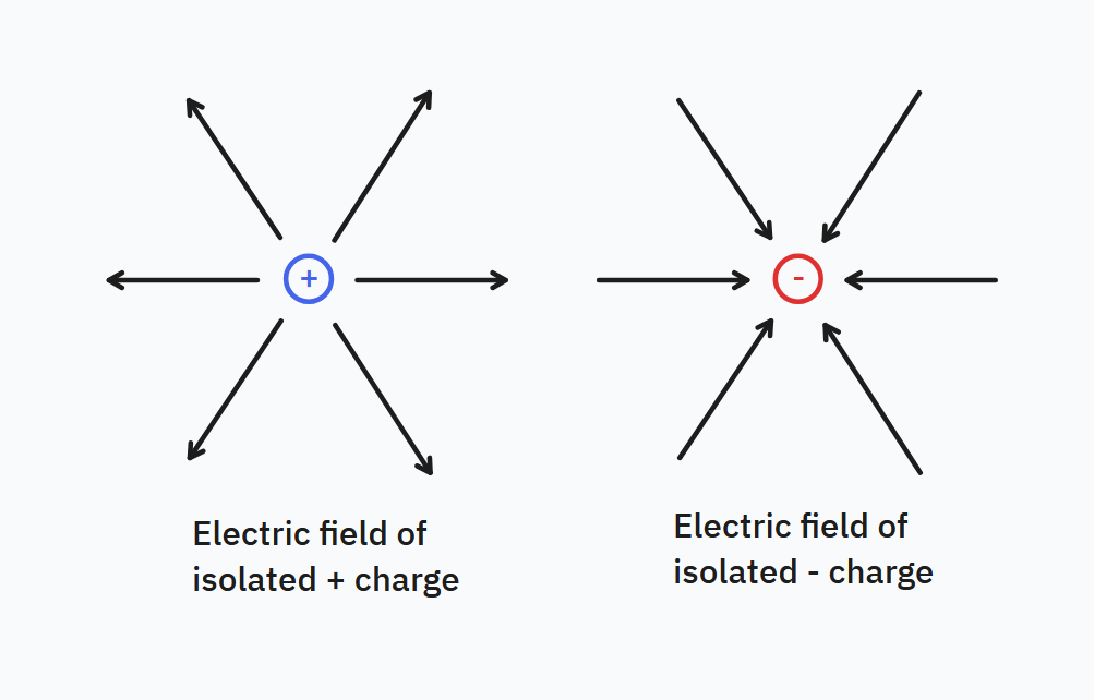
For the advanced reader: later on the fact that electric field vectors point inwards towards negative charges and outwards towards positive charges becomes associated with the nature of electrical potential energy. Specifically, the electromagnetic potential energy descends down from positive charges to negative charges; higher regions of potential energy push (accelerate) particles away from them to descend down to lower regions. The field analogue of the potential energy is the potential $V$ and for electrostatics it obeys $\mathbf{E} = -\nabla V$.
Electric fields from one charge and another charge sum; this is known as superposition. The general expression for the electric field produced from a collection of $n$ charges $q_1, q_2, q_3, \dots q_n$ is given by:
$$ \mathbf{E}(x, y, z) = \sum_i \frac{q_i}{4\pi \epsilon_0} \frac{(x-x_i)\hat{\mathbf{i}} + (y-y_i)\hat{\mathbf{j}}+ (z-z_i)\hat{\mathbf{k}}}{((x-x_i)^2 + (y-y_i)^2 + (z-z_i)^2)^{3 \over 2}} $$
Where $(x_i, y_i, z_i)$ are the position of each of the charges and $(x, y, z)$ is the position of a point in space. Note that both for the discrete single-charge and multiple-charge case, these equations for the $\mathbf{E}$ are only valid for localized charges (i.e. when charges can be considered approximately pointlike). Point charges do not exist in the real world and the whole expression blows up at $r = 0$, so rather these equations for the field are approximate for a distance $r \gg 0$ that is far from the charges.
Note of nuance for the advanced reader: We will later see that by Gauss's law, any spherically-symmetric distribution of charge (such as a sphere of charge) acts as if all of its charge were concentrated at its center, i.e. act the same as point charges. This means that non-point particles do exactly follow Coulomb's law so long as they are spherically-symmetric. In addition, protons and electrons do indeed act similar (but not exactly) like point particles, or at least can be treated as such. So this is not as bad of an approximation as it may seem.
Other formulations for the electric field produced by discrete charges
We may write the electric field produced by discrete charges in a simpler fashion as follows:
$$ \mathbf{E}(x, y, z) = \sum_i \frac{q_i}{4\pi \epsilon_0} \frac{1}{(r-r_i)^2} \hat{\mathbf{r}} $$
Where $\hat{\mathbf{r}}$ is the unit vector of the vector $\langle x-x_i, y-y_i, z-z_i\rangle$, and $r = |\langle x-x_i, y-y_i, z-z_i\rangle| = \sqrt{(x-x_i)^2 + (y-y_i)^2 + (z-z_i)^2}$ is the distance from a point $(x, y,z)$ in space and $(x_i, y_i, z_i)$. We may show this with:
$$ \begin{align*} \mathbf{E}(x, y, z) &= \sum_i \frac{q_i}{4\pi \epsilon_0} \frac{(x-x_i)\hat{\mathbf{i}} + (y-y_i)\hat{\mathbf{j}}+ (z-z_i)\hat{\mathbf{k}}}{((x-x_i)^2 + (y-y_i)^2 + (z-z_i)^2)^{3 \over 2}} \\ &= \sum_i \frac{q_i}{4\pi \epsilon_0} \frac{\langle x-x_i, y-y_i, z-z_i\rangle}{((x-x_i)^2 + (y-y_i)^2 + (z-z_i)^2)^{3 \over 2}} \\ &= \sum_i \frac{q_i}{4\pi \epsilon_0} \frac{\|\langle x-x_i, y-y_i, z-z_i\rangle\|}{((x-x_i)^2 + (y-y_i)^2 + (z-z_i)^2)^{3 \over 2}} \hat{\mathbf{r}} \\ &= \sum_i \frac{q_i}{4\pi \epsilon_0} \frac{r-r_i}{(r - r_i)^\frac{3}{2}} \hat{\mathbf{r}} \\ &= \sum_i \frac{q_i}{4\pi \epsilon_0} \frac{1}{(r - r_i)^2} \hat{\mathbf{r}} \end{align*} $$
This formulation is also very useful when there are symmetries in the field that simplify the formulation of the field, and also for simplicity when there is a simple expression for $r$. Note, however, that this involves care in ensuring that the unit vector $\hat{\mathbf{x}} = \dfrac{\langle x - x_i, y - y_i, z - z_i\rangle }{\| \langle x - x_i, y - y_i, z- z_i\rangle \|}$ is chosen correctly, because $\hat{\mathbf{r}}$ is not the same as the Cartesian space unit vector $\hat r = \hat x + \hat y + \hat z$, which it can easily be confused with.
Continuous distributions of charges
We have seen the case of a discrete distribution of static charges $q_1, q_2, q_3, \dots$ located at positions $(x_1, y_1, z_1), (x_2, y_2, z_2), \dots$, the electric field is given by:
$$ \mathbf{E}(x, y, z) = \sum_i \frac{q_i}{4\pi \epsilon_0} \frac{(x-x_i)\hat{\mathbf{i}} + (y-y_i)\hat{\mathbf{j}}+ (z-z_i)\hat{\mathbf{k}}}{((x-x_i)^2 + (y-y_i)^2 + (z-z_i)^2)^{3/2}} $$
So long as we consider all the charges in the superposition of charges, then the electric field contains the contribution of every charge and knowledge of the electric field uniquely determines the motion of each charge in the system for all times $t$ by $\mathbf{F} = m \ddot{\mathbf{r}} = q\mathbf{E}$; unlike Newtonian mechanics, there is no need to compute all the inter-particle forces to find the equations of motion.
One unique feature of electric fields is that the electric field magnitude at each point only depends on the position of each charge and the total charge in the system, given by the sum of the absolute value of each charge. Neither the sign of each of the charges, or the vector direction of the electric field, have any effect on the electric field's magnitude (though they do impact the direction).
Consider a distribution of static charges arranged throughout space such that we may model all the charges as a single object of continuous density function. This may be a curved metal rod that contains a great number of static charges (electrons), such that the object may be modelled as a continuous distribution of charge. Remember that for continuous problems, we must use integration. In integral form, the electric field caused by a continuous and non-uniform distribution of charges is given by:
$$ \begin{align*} \mathbf{E}(x, y, z) &= \frac{1}{4\pi \epsilon_0} \int \frac{(x-x')\hat{\mathbf{i}} + (y-y')\hat{\mathbf{j}}+ (z-z')\hat{\mathbf{k}}}{\left[(x-x')^2 + (y-y')^2+ (z-z')^2\right]^{3/2}} dq' \\ &= \frac{1}{4\pi \epsilon_0} \int \frac{\mathbf{r} - \mathbf{r}'}{\|\mathbf{r} - \mathbf{r}'\|^3} dq' \end{align*} $$
This expression may seem very complex and confusing; therefore it must be clarified as follows:
- $\mathbf{r} = \langle x, y, z \rangle$ denotes a point in 3D space at $(x, y, z)$ from which the field is measured, which can be chosen arbitrarily when computing the integral. This is the same $x, y, z$ as in $\mathbf{E}(x, y, z)$.
- $\mathbf{r}' = \langle x', y', z'\rangle$ denotes the location of an infinitesimal element (e.g. line element, surface element, volume element) along the object of continuous charge, which is integrated over the entire object.
- $dq' = \lambda dx' = \sigma dA' = \rho dV'$ where $dx', dA', dV'$ are the line element, surface element, and volume element respectively along the coordinates $(x', y', z')$, and substitution of one of these is necessary to be able to solve the integral explicitly.
Mathematical interlude: some texts use the notation $| \mathbf{r} - \mathbf{r}'|$ instead, this is functionally equivalent to $\|\mathbf{r} - \mathbf{r}' \|$ because of the vector identity $| \mathbf{v} | = \sqrt{v^2} = \sqrt{\mathbf{v} \cdot \mathbf{v}} = \| \mathbf{v}\|$. We will use both interchangeably.
Visually, we may represent the integration process as shown in the below diagram:

Note that these equations apply only for static fields (i.e. unchanging with time). The integrals in general are non-trivial and can only be solved numerically, but symmetries in the problem may simply the integral sufficiently to be solved analytically.
In practice, due to the difficulties of modelling, when there is a dominant charged object, we often consider only the contribution of a single object and consider the other charges as contributing negligibly to the field. This technically does not model the problem exactly but approximately holds. This is analogous as the classical field theory of Newtonian gravity, where the common approximation $\displaystyle \mathbf{g} = -\frac{GM_\mathrm{sun}}{r^2} \hat r$ is approximately true and yields the correct orbits if one uses it to solve for the gravitational field (and thus orbits of planets) within the solar system, since the Sun is so much more massive than all the planets.
Note for the advanced reader: We can, in fact, model multiple charged objects that are each continuous charge distributions but separated by space, such as several non-uniform metal shapes. In this case for $N$ objects that have varying charge distributions that are separated by space we may use the Dirac delta "function" (it technically is not a function but can be treated as a function by:
$$ \mathbf{E}(x, y, z) = \frac{1}{4\pi \epsilon_0} \int \sum_{i=1}^N \frac{\delta(\mathbf{r} - \mathbf{r}_i')}{\|\mathbf{r} - \mathbf{r}_i'\|^{3/2}} \,dq_i' $$
There are some symmetries that can be used to simplify the integral in special cases:
- The electric field is always zero within a conductor, even when placed beside a charged object, because the mutual attraction and repulsion of electrons cancels out
- The electric field is always zero within a spherically-symmetric shell of charge (we'll see why later when we study Gauss's law)
- The electric field outside a spherically-symmetric object is equivalent to $\mathbf{E} = \frac{kQ}{r^2} \hat r$ even if the interior charge density is non-uniform; this holds as long as the interior charge density is spherically symmetric.
Other formulations for the electric field produced by continuous charges
In many cases, the symmetries of a problem lead to some of the components of the electric field canceling out. Therefore, it is often more helpful to use the alternative component-valued formulation, and only solve for the nonzero components:
$$ \begin{align*} E_x = \frac{1}{4\pi \epsilon_0} \int \frac{x-x'}{\left[(x-x')^2 + (y-y')^2+ (z-z')^2\right]^{3/2}} dq' \\ E_y = \frac{1}{4\pi \epsilon_0} \int \frac{y - y'}{\left[(x-x')^2 + (y-y')^2+ (z-z')^2\right]^{3/2}} dq' \\ E_z = \frac{1}{4\pi \epsilon_0} \int \frac{z-z'}{\left[(x-x')^2 + (y-y')^2+ (z-z')^2\right]^{3/2}} dq' \end{align*} $$
Problems analytically solvable by Coulomb's law
Electric field of a charge (monopole)
The electric field produced by a single charge $Q$ is by definition given by:
$$ \mathbf{E} = \frac{kQ}{r^2} \hat r = \frac{1}{4\pi \epsilon_0} \frac{Q}{r^2} \hat r $$
Electric field of a dipole
Consider two charges $q_1, q_2$ at $(x_1, y_1, z_1)$ and $(x_2, y_2, z_2)$. This is a good approximation for various molecules that have a positively charged and negative charged end (see this PDF to read more about this). We use the superposition principle and just add up the respective electric fields of each charge to obtain:
$$ \begin{align*} E_x = \frac{1}{4\pi \epsilon_0} \left(\frac{q_1(x - x_1)}{\left(x - x_1)^2 + (y - y_1)^2 + (z - z_1)^2\right)^{3/2}} + \frac{q_2(x - x_2)}{\left(x - x_2)^2 + (y - y_2)^2 + (z - z_2)^2\right)^{3/2}}\right) \\ E_y = \frac{1}{4\pi \epsilon_0} \left(\frac{q_1(y - y_1)}{\left(x - x_1)^2 + (y - y_1)^2 + (z - z_1)^2\right)^{3/2}} + \frac{q_2(y - y_2)}{\left(x - x_2)^2 + (y - y_2)^2 + (z - z_2)^2\right)^{3/2}}\right) \\ E_z = \frac{1}{4\pi \epsilon_0} \left(\frac{q_1(z - z_1)}{\left(x - x_1)^2 + (y - y_1)^2 + (z - z_1)^2\right)^{3/2}} + \frac{q_2(z - z_2)}{\left(x - x_2)^2 + (y - y_2)^2 + (z - z_2)^2\right)^{3/2}}\right) \end{align*} $$
For the electrical field of an electrical dipole, the fields of the charges cancel outside the charge of the smaller magnitude (here we refer to the space between the charge as the inside, and the opposite space, directed away from each charge towards infinity, as the outside).
Conductors, dielectrics, and polarization
Materials respond differently when they are placed within an electric field. In conductors, where charges are free to move,
A dielectric is a material that is (roughly speaking) composed of bound positive and negative charges. When an external electric field (such as that of a charged rod) is placed near a dielectric, negative charges will feel a force against the direction of the field. Therefore, the negatively charges within the insulator orient themselves against the field, and the positive charges orient themselves towards the field. But since all electrons are bound tightly to their atoms in dielectrics, the charges cannot redistribute themselves to make the overall charge neutral; thus the dielectric exhibits all the same effects of polarization. That is to say, while no charges can flow through a dielectric, it nonetheless has an inner electric field (also called polarization field, denoted $\mathbf{D}$) and is considered polarized. Note that while all dielectrics are insulators, not all insulators are dielectrics because not all insulators have polar molecules (roughly, bound positive and negative charges). A dielectric need not be a material at all; a vacuum is technically a dielectric because an externally applied electric field creates an inner electric field within the vacuum.
We characterize dielectrics by a dielectric constant $\kappa$, where $\kappa = \dfrac{E_0}{E}$, $E_0$ is the electric field if the dielectric was not present, and $E$ is the actual electric field. With a known dielectric constant, and a known electric field configuration in the absence of a dielectric, we can therefore find the actual electric field by $E = \dfrac{E_0}{\kappa}$.
The electric field inside a conductor must be zero, no matter the charge(s) placed within it. Therefore, if the said conductor is a shell, the inner surface charge of such a conductor will equal the total charge placed within the conductor, such that the electric field produced by inner charges and the inner surface charge cancels out and therefore the net electric field inside the conductor is zero. Even when a conductor is polarized, no electric field develops in the conductor, because the charges within redistribute themselves so that the electric field from the charges exactly cancels out the external field so that the interior field is zero. The electric field outside a polarized conductor (really, for any conductor) can be very nontrivial, but the electric field inside is always, always zero.
Gauss's law
We will now introduce another method to calculate the electric field: Gauss's law. Gauss's law relates the flux $\Phi_E$ (directional spread) of an electric field within a region of space to the total charge enclosed by an (imaginary) shape in that region of space:
$$ \Phi_E =\oint\limits_\mathrm{closed} \mathbf{E} \cdot \, d\mathbf{A} = \frac{Q_\mathrm{enclosed}}{\epsilon_0} $$
The imaginary enclosing surface is called a Gaussian surface. It must be a closed three-dimensional surface, meaning that all electric field vectors that come from electric fields inside the surface must "pass through" Gaussian surface. This also means that the Gaussian surface must enclose any charges that are within it, and have no holes.
Here, $d\mathbf{A} = \hat{\mathbf{n}}, dA$ is an infinitesimal patch of the shape's surface, $\hat{\mathbf{n}}$ is the normal vector to that patch and the circled integral is a surface integral over the surface of the shape. For instance, if the shape was a square, then $d\mathbf{A} = \hat{\mathbf{n}},dx,dy$; if the shape was a sphere, then $d\mathbf{A} = 4\pi r^2 \hat{\mathbf{n}} dr$ (from the surface area formula of a sphere. In the general case, the flux can be visualized as follows:

Original source: Wikipedia
Note for the advanced reader: in alternate (typically more advanced) formulations Gauss's law can be equivalently written in terms of the charge density and the Coulomb constant:
$$ \oint \limits_{\partial \Omega} \mathbf{E} \cdot d\mathbf{A} = 4\pi k \iiint \limits_\Omega \rho\, dV $$
In some cases with symmetries, Gauss's law is able to simplify calculations for the electric field as compared to integration by Coulomb's law. While remaining an integral equation, three specific symmetries for the electric field lead to straightforward analytical expressions: spherical, cylindrical, and planar. For example, consider a point charge $Q$ surrounded by an (imaginary) sphere of radius $r$. By Gauss's law we have:
$$ \oint\limits_\mathrm{closed} \mathbf{E} \cdot \, d\mathbf{A} = \oint\limits_\mathrm{closed} \mathbf{E} \cdot \, 4\pi r^2\, \hat{\mathbf{n}}\,dr $$
The normal vector to the sphere's surface is given by $\hat r$ and the electric field also spreads spherically outwards, that is, $\mathbf{E} = E, \hat r$. Thus, the dot product is equal to one, as shown:
$$ \oint\limits_\mathrm{closed} E\, \hat r \cdot \, 4\pi r^2\, \hat{\mathbf{n}}\,dr $$
In addition, the flux within a Gaussian sphere surrounding any spherically symmetric charge or charge distribution is always $\Phi(r) = E, 4\pi r^2$ for any spherically symmetric object. This is because the normal vectors and electric field vectors both point along $\hat r$.
When applying Gauss's law, there are a lot of specific areas to take notice, lest they mess up your calculation:
- Gauss's law does not apply to a non-closed surface.
- Gauss's law is typically not analytically computable when a surface has non-constant normal vectors
- Gauss's law works by taking one region of the field and the integrating over the surface of that region, which then equates the field globally so long as the field is symmetric. That is why it works even for infinitely long wires or infinitely large diameter sheets, because we can surround the electric field in a finite region and integrate over the finite charge within that region. Remember that you are only considering the enclosed charge, not the total charge (which may very well be infinite for infinitely long wires and sheets)
Several important facts about Gauss's law are very counterintuitive, so we will go over them in detail. The first is that while there is zero electric field within a Gaussian surface of zero enclosed charge, this does not mean there are no charges within the Gaussian surface. There may certainly be charges that cancel out each other, resulting in zero net charge, but nonzero regions of charge. That is to say:
Zero electric field does not necessarily imply zero charge within the Gaussian surface.
The second fact is that nothing outside a Gaussian surface, even the presence of other charges and external fields, can affect the electric field inside a Gaussian surface. This is because the flux of any external electric field across a closed Gaussian surface is always zero. An external electric field is not possible to be enclosed in a closed surface, so by definition it has no effect. To summarize:
External fields outside a Gaussian surface have no effect on the field within the Gaussian surface.
Finally, simply knowing the electric field within a Gaussian surface does not tell you anything about the electric field outside the Gaussian surface, except in one specific case. The electric field outside the surface of a charged conductor has field lines that are always perpendicular to the surface. The magnitude, however, can be anything, and this is not true in the general case of a non-conductor.
Problems analytically solvable via Gauss's law
For a problem to be reasonably solvable by Gauss's law, the geometry of the problem should be such that it satisfies two conditions:
- A Gaussian surface may be found whose surface normals are directly parallel to the electric field vectors
- The field is constant through the Gaussian surface. This means that the electric field is independent of the Gaussian surface.
Due to this reason, complex geometries and electric fields are not typically analytically solvable by Gauss's law and must be numerically computed. However, approximate expressions for the electric field can be found and be used as a starting point for higher-order corrections.
Infinitely-long conducting rod
This may be used, for instance, to model the electric field generated by an infinitely-long wire of uniform charge density $\lambda$. The Gaussian surface used is an (imaginary) cylinder of radius $r$ coaxial to the rod. We consider a segment of the wire with length $L$. Therefore the total charge within that segment is $Q = \lambda L$. The cylindrical Gaussian surface surrounding that segment of wire has surface area $2\pi r L + 2\pi r^2$, but as the electric field vectors are orthogonal to the normal vectors at the caps, their contributions are zero, and thus the effective surface area is simply $2\pi rL$. Therefore Gauss's law takes the form:
$$ \oint \limits_{\mathrm{cylinder}} E(2\pi rL) = \frac{\lambda L}{\epsilon_0} $$
After rearranging we obtain:
$$ \mathbf{E} = \frac{\lambda}{2\pi r\epsilon_0} \hat r $$
Note that the electric field of an infinite cylinder of charge can be obtained using similar methods and has a similar result.
Infinite double-sided sheet of charge
We can use this to model the electric field of any suitably flat surface of charge with uniform surface charge density $\sigma$. The Gaussian surface used is an (imaginary) cylinder of radius $R$ and height $h$, which is aligned vertically. The electric field vectors align with the flat top caps and bottom caps of the cylinder. Thus the total surface area $S_A = 2\pi rL + 2\pi R^2$ has only the contributions from the caps, and the effective surface area is $S_A = 2\pi R^2$. Meanwhile, the enclosed charge would be a circle of charge on the sheet enclosed by the cylinder of area $A = \pi R^2$ and thus we have:
$$ \oint \mathbf{E} \cdot d\mathbf{A} = 2\pi R^2 E = \frac{\sigma A}{\epsilon_0} = \frac{\pi R^2 \sigma}{\epsilon_0} $$
And thus:
$$ \mathbf{E} = \frac{\sigma}{2\epsilon_0} \hat z $$
Note that this is the same expression as the electric field near the center of a double-sided disk of charge, where the disk is of radius $R$ and has surface charge density $\sigma$ (in the single-sided disk of charge case, the electric field is double that, so $\mathbf{E} = \dfrac{\sigma}{\epsilon_0}\hat z$). This only holds near the center of the disk, however; it is an approximate expression for the case that $r \ll R$.
Infinite single-sided sheet of charge
An infinite single-sided sheet of charge is a good approximation for the electric field of any charged surface that can be considered relatively flat and large. The calculations are the same as the double-sided case but we only consider one side, and therefore the effective surface area is one-half that of the previous, and thus $S_A = \pi R^2$. In this case:
$$ \mathbf{E} = \frac{\sigma}{\epsilon_0} \hat z $$
Additionally, by a similar argument, we may show that the electric field between two charged plates both of uniform surface charge density is also $\mathbf{E} = \dfrac{\sigma}{\epsilon_0}\hat z$.
Near surface of an ideal conductor
This is equal to an infinite single-sided sheet of charge, because the electric field near the surface of an ideal conductor is approximately flat and therefore (approximately) equal to that of an infinite single-sided sheet of charge. Therefore:
$$ \mathbf{E} = \frac{\sigma}{\epsilon_0} \hat z $$
Inside a spherical insulating sphere
We consider the electric field inside a spherically insulating sphere of uniform charge density $\rho$. Note that this is not the same as that of the electric field outside the sphere $\mathbf{E} = \dfrac{kq}{r^2} \hat r$. In this case the total charge within the sphere at radius $r$ becomes $Q(r) = \rho V(r) = \dfrac{4}{3} \pi r^3 \rho$ (where $V(r)$ is the volume at distance $r$ from the center of the sphere, not the electrical potential) and thus the electric field is $\mathbf{E} = \dfrac{\rho r}{3 \epsilon_0} \hat r$.
Note that the electric field inside a spherical conducting sphere is simply zero, and likewise for a spherical shell of charge.
Outside a conducting infinitely-long cylinder
We may surround a conducting infinitely-long cylinder of uniform linear charge density $\lambda$ with a cylindrical Gaussian surface with radius $r$ and length $L$, and therefore the enclosed charge becomes $Q_\mathrm{enc.} = \lambda L$. Thus, by Gauss's law:
$$ \oint \mathbf{E} \cdot d\mathbf{A} = 2\pi rL E = \frac{\lambda L}{\epsilon_0} $$
By rearranging we get:
$$ \mathbf{E} = \dfrac{\sigma}{2\pi r \epsilon_0} \hat r $$
Electrical potential energy
The electrical potential energy is the energy stored within the electric field generated by a system of charges that can be released for charges to move. Electric potential energy is always defined against a specific reference point; if we define the electrical potential energy to be zero at infinity, then two charges brought towards each other a distance $r$ apart would have an electric potential energy $U_E$ of the following:
$$ U_E = \dfrac{kq_1 q_2}{r} $$
For a system of $N$ charges $q_1, q_2, \dots q_N$ and defining relative to infinity, the expression for the electric potential energy is given by:
$$ U_E = \frac{1}{2} \sum_{i = 1}^N \sum_{j = 1}^N \frac{kq_i q_j}{r_{ij}} $$
However, this is not a very useful formula as it is quite verbose. Rather, it is more useful to use another (more conceptual) approach. Suppose we had a system of three charges, with the magnitude of each charge being $Q$, arranged in an equilateral triangle of side lengths $L$:

We aim to obtain the electric potential energy of the system; that is, how much energy is stored in the system of charges if we consider the energy to be zero at infinity, which is important when considering problems that are solved using the conservation of energy.
To do so, we consider the process of bringing in each charge one by one, as illustrated below (the charges have been color-coded for clarity):

In the first step, the first charge is brought from infinity. There is nothing to resist its motion, and therefore the contribution to the potential energy is zero. In the second step, the second charge is brough from infinity to join the system. As it is oppositely charged, the potential energy is negative, meaning that energy must be put into the system to keep the charges separate. Since there are only two charges, $Q$ and $-Q$, the contribution to the potential energy in the second step step is $\dfrac{k(Q)(-Q)}{r} = -\dfrac{kQ^2}{L}$ by application of the electric potential energy formula. In the third step, the third charge is brought from infinity. Its interaction with the existing two-charge system results in a potential energy of $\dfrac{kQ^2}{L}$ with the red charge $+Q$ (the positive charge in the two-charge system) and $-\dfrac{kQ^2}{L}$ with the purple charge $-Q$ (the negative charge in the two-charge system). Therefore the total potential energy contributed by the third step is the sum of these potential energies, i.e. $\dfrac{kQ^2}{L} + \left(-\dfrac{kQ^2}{L}\right) = 0$. Thus the total electrical potential energy is the sum of the potential energy contributions by each of the three steps, that is:
$$ U_\mathrm{E}^{(\mathrm{total})} = U_1 + U_2 + U_3 = 0 + -\dfrac{kQ^2}{L} + 0 = -\dfrac{kQ^2}{L} $$
And thus we arrive at the result. This method is generalizable to any configuration of discrete charges.
Electric potential
In electrostatics, we may define another field called the electric potential as the following line integral:
$$ V(r) = -\int_{C[r_0 \to r]} \mathbf{E} \cdot d\mathbf{r} = -\int_{r_0}^r \mathbf{E} \cdot d\mathbf{r} $$
Where $r = (x, y, z)$ is a shorthand and $d\mathbf{r}$ is an infinitesimal segment of the parametric curve $C$ from $r_0$ to $r$. This definition is probably too abstract, so here is a more intuitive explanation.
Particles possess energy in one of two forms; either energy in motion (kinetic energy) or energy that is stored in some way (battery, rubber band, etc.). The second form - stored energy that has not been used - we refer to as potential energy. When an object is allowed to freely move, it loses its stored energy (potential energy). This is because you can never create more energy, as energy is conserved, so (kinetic) energy in motion necessarily decreases stored (potential) energy.
In electromagnetism, the electric field acts as a store and carrier of energy. Charges placed in the electric field gain energy, almost like a phone being plugged into a charging cable. The electric potential $V(r)$ is the field proportional to the potential energy within the electric field. Where the potential has a higher value, particles have more potential energy; where the potential has a lower value, particles have less potential energy.
But stable configurations in nature are the lowest potential energy configurations. So charges immediately try to get to the lowest potential energy point possible. As the charge moves within the electric field $\mathbf{E}$, it takes the path $\mathbf{r}(t)$ that will help it minimize its potential energy.
We can therefore integrate along the path from the charge's original point $r$ to the point of zero potential energy $r_0$ (as in "ground point" or "zero point"), as follows, to find the total decrease in potential energy $\Delta U$:
$$ \Delta U = \int_r^{r_0} q\mathbf{E} \cdot d\mathbf{r} $$
To find the original potential energy $U$ of the charge $q$ at point $r$, we simply work backwards, from $r_0$ to $r$, so we have:
$$ \begin{align*} U_{\text{at } r} - \Delta U &= U_{\text{at } r_0} \\ &\Rightarrow U_{\text{at } r} = \cancel{U_{\text{at } r_0}}^0 + \int_r^{r_0} q\mathbf{E} \cdot d\mathbf{r} \end{align*} $$
But since we want this expression to show that we are finding the energy at $r$ relative to $r_0$ (which is mathematically identical but physically different), we can use the bound-switching property of integrals to rewrite as:
$$ \int_r^{r_0} q\mathbf{E} \cdot d\mathbf{r} = -\int_{r_0}^r q\mathbf{E} \cdot d\mathbf{r} $$
We can then define the potential field $V(r) = U / q$, which gives the potential energy a charge would gain at every point in space, relative to a lowest energy point $r_0$:
$$ V(r) = -\int_{r_0}^r \mathbf{E} \cdot d\mathbf{r} $$
Careful! Here, $V(r)$ is a field, so we write it as a function of $r$, but $U$ is an energy value relative to some point (usually infinity) so do not consider it as a function and do not write it as $U(r)$ even if it is sometimes mathematically convenient. It is better to write $U_r$ or (the somewhat clumsy) $U_{\text{at } r}$, after specifying where the zero point of the potential is Remember, adding a constant to the potential energy doesn't change the electric field. It is a good idea to explicitly write out, for instance, that $U$ is the potential energy relative to a point where it is zero, located infinitely far away.
Unlike electrical potential energy $U$, which is the potential energy of a charge (relative to some predefined zero point) and is a single number, the electrical potential is a field quantity, described by a function, and defined at every point $r$ in space. This is why we describe it as a field proportional to the potential energy within the electric field. Mathematically, we say that $U_E = q V(r)$ where $U_E$ is the potential energy of a charge $q$ at point $r$, relative to a zero point $r_0$.
A useful visualization: One can visualize an electrical potential as a landscape with hills and valleys. A positive charge is like a ball placed onto such a landscape; the direction it will move in is towards the direction of lowest potential, which would be like rolling down the hill. A negative charge is like a ball that sees the landscape upside-down, so it rolls up the hill, because it sees everything flipped upside-down and thinks the hill is actually going down.
The line integral is notably path-independent such that integrating any path between $r_0 \to r$ yields the same result, and therefore the simplest path is preferred for calculational convenience.
It is by common convention that when $r_0$ is not explicitly given, we may define the reference point $r_0$ to be infinitely far away, such that the potential vanishes at infinity $V_\infty = 0$. Then the potential becomes:
$$ V(r) = -\int_\infty^r \mathbf{E} \cdot d\tilde{\mathbf{r}} $$
Where $d\tilde{\mathbf{r}}$ is still an infinitesimal curve segment, exactly the same as $d\mathbf{r}$, the switch in symbol is simply to avoid conflict with the $r$ in the integration bounds. With this definition, the electrical potential generated by a point charge at position $(0, 0, 0)$ is:
$$ V(r) = -\int_\infty^r \frac{kq}{\tilde r^2}\, d\tilde r = \frac{kq}{r}, \quad r > 0 $$
The electric potential, like the electric field, obeys the principle of superposition, such that the respective potentials of multiple charges sum together:
$$ V(r) = \frac{1}{4\pi \epsilon_0} \sum_i \frac{q_i}{r_i} $$
And in the continuous case, the summation becomes an integral over a charge distribution:
$$ V(r) = \frac{1}{4\pi \epsilon_0} \int \frac{1}{|r - r'|} \,dq' $$
As an example, consider a finite line charge of length $L$. We wish to calculate the potential at distance $x$ from the end of the line charge. In this case $dq = \lambda dx'$ and $|r - r'| = |x + x'|$ such that:
$$ V = \frac{1}{4\pi \epsilon_0} \int \frac{\lambda dx'}{|x + x'|} = \frac{\lambda}{4\pi \epsilon_0} \ln \left(\frac{x + L}{x}\right) $$
If we have three points arranged such that $a > b > c$, the electric potential at point $c$ relative to point $a$ is equal to the sum of the electric potential at point $b$ (relative to point $a$) and the electric potential at point $c$ relative to point $b$. This clumsily-worded sentence can be much better be expressed mathematically:
$$ \begin{align*} V(c) &= -\int_a^b \mathbf{E} \cdot d\mathbf{r} + V(b) \\ &=\left(-\int_a^b \mathbf{E} \cdot d\mathbf{r}\right) + \left(-\int_b^c \mathbf{E} \cdot d\mathbf{r}\right) \\ &= \int_b^a \mathbf{E} \cdot d\mathbf{r} + \int_c^b \mathbf{E} \cdot d\mathbf{r} \end{align*} $$
This is very useful, for instance, in deriving the electric potential within a sphere of radius $R$, where we must add up the electric potential at the surface of the sphere given by $V_0 = \dfrac{kq}{R}$ to find the expression of the total electric potential within the sphere $V(r) = -\displaystyle\int_R^r \mathbf{E} \cdot d\mathbf{r} + V_0$ which evaluates to $V(r) = V_0 + \dfrac{\rho(R^2 - r^2)}{6\epsilon_0}$.
From the definition of the electrical potential, we may define the potential difference (more commonly called voltage) as the difference in the electrical potential between two points $a$ and $b$:
$$ \Delta V = V(b) - V(a) $$
Which we may also write via the line integral definition of the electrical potential:
$$ \Delta V = -\int_a^b \mathbf{E} \cdot d\mathbf{r} $$
This is the same type of voltage as marked on household batteries; the nonzero voltage means that one end of the battery is at a higher potential as compared to the other end, so charges flow away from the higher-potential end to the lower-potential end. The electric potential energy $U$ of a charge at a point $(x, y, z)$ is related to the electrical potential by $U = qV$. Similarly, $\Delta U = q\Delta V$.
Additionally, the electric field can be computed from the electrical potential by taking the derivative of the electric potential in every coordinate direction. This uses the gradient (nabla) operator from vector calculus, as shown below:
$$ \mathbf{E} = -\nabla V = -\left(\frac{\partial V}{\partial x} \hat{\mathbf{i}} + \frac{\partial V}{\partial y} \hat{\mathbf{j}} + \frac{\partial V}{\partial z} \hat{\mathbf{k}}\right) $$
In physical terms, this represents the fact that an electric field develops between regions of differing electrical potential, as charges, which form electric fields, are naturally pushed away from high potential regions and descend towards low potential regions. We say that the two regions have a potential gradient and therefore there is a nonzero electric field present between the regions.
We presume that the charges are positive in this case. A negative charge would exhibit the opposite behavior, i.e. be pushed away from low potential regions and drawn toward higher potential regions.
This is one of the most useful characteristics of the electric potential as knowledge of the electric potential uniquely determines the associated electrical field. We may graphically illustrate this fact by drawing isolines, which represent equipotential surfaces (surfaces of constant electrical potential). One such drawing is shown below:
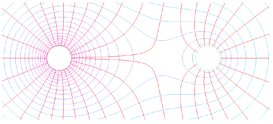
Credit: TeX Stack Exchange
Electrical field lines run across and perpendicular to equipotential surfaces, and electric fields exert forces on charges, so the trajectories of charges can simply be drawn by tracing curves perpendicular to the isolines. Note that the surface of an electrical conductor is always an equipotential surface due to the fact that the electric field within any electrical conductor is always zero. In addition, every Gaussian surface drawn in a conductor would also be an equipotential surface. We may state this fact as follows:
The electric potential on the surface and inside a conductor always forms an equipotential surface (i.e. has the same potential everywhere on the surface). Furthermore, the electric potential is constant on the surface of and within a conductor.
Note for the advanced reader: the electrical potential can also be understood through the electrostatic Poisson equation $\nabla^2 V = -4\pi k \rho$, where a conductor can be thought of as a specific Dirichlet boundary-value problem, for which that has the unique solution $V = C$ i.e. $V$ is a constant. More on this later.
A brief vector calculus interlude
To continue our discussion of electromagnetism, it is helpful to take a brief look at vector calculus, which is the branch of calculus specialized to the study of vector and scalar fields used extensivley in electromagnetic theory.
Gradient
The gradient of a scalar-valued function, denoted $\nabla f$, is given by a vector containing all the partial derivatives of the function. In two dimensions, it is given by:
$$ \nabla f(x, y) = \left\langle \frac{\partial f}{\partial x}, \frac{\partial f}{\partial y} \right\rangle $$
In three dimensions, it is similarly given by:
$$ \nabla f(x, y, z) = \left\langle \frac{\partial f}{\partial x}, \frac{\partial f}{\partial y}, \frac{\partial f}{\partial z} \right\rangle $$
The gradient can be evaluated at a point $(x, y, z)$ by evaluating each of the partial derivatives at that point
Divergence
Divergence, denoted by $\nabla \cdot \mathbf{F}$, represents the tendency of a vector field to flow out or in to a certain point:
- If vectors that point inwards towards a certain point are bigger than vectors that point outwards at that point, the divergence is negative, and we have a sink
- If vectors that point inwards towards a certain point are smaller than vectors that point outwards at that point, the divergence is positive, and we have a source
- If vectors that point inwards and vectors that point outwards at a certain point are equal in size, the divergence is zero
The divergence of a vector field $\vec F$ with components $\langle F_x, F_y, F_z\rangle$ is given by:
$$ \nabla \cdot \vec F = \frac{\partial F_x}{\partial x} + \frac{\partial F_y}{\partial y} + \frac{\partial F_z}{\partial z} $$
Divergence is only defined on vector fields, not on scalar fields.
Curl
Curl, denoted by $\nabla \times \vec F$, represents the tendency of a vector field to rotate around a certain point:
- Positive curl is a tendency of vectors to rotate counterclockwise around a point
- Negative curl is a tendency of vectors to rotate clockwise around a point
- Zero curl is when counterclockwise and clockwise vectors cancel out or if the vectors do not rotate around a point
- As the curl of a vector field is another vector field, we can say that in a physical setting, taking the curl of a vector field produces a new circulating vector field (this will become relevant when studying the 3rd and 4th Maxwell equations)
In 2D, the curl of a vector field is given by:
$$ \nabla \times \vec F = \frac{\partial F_y}{\partial x} - \frac{\partial F_x}{\partial y} $$
In 3D, the curl of a vector field is the determinant of a 3 x 3 matrix:
$$ \nabla \times \vec F = \begin{vmatrix} \hat i & \hat j & \hat k \\ \frac{\partial}{\partial x} & \frac{\partial}{\partial y} & \frac{\partial}{\partial z} \\ F_x & F_y & F_z \end{vmatrix} $$
Laplacian
The Laplacian, denoted by $\nabla^2 f$, is a scalar field formed from the second derivatives of a scalar field. It is given by:
$$ \nabla^2 f = \frac{\partial^2 f}{\partial x^2} + \frac{\partial^2 f}{\partial y^2} + \frac{\partial^2 f}{\partial z^2} $$
A function is called harmonic if it satisfies $\nabla^2 f = 0$. This is a partial differential equation called Laplace's equation.
The divergence theorem
$$ \oint \mathbf{E} \cdot d\mathbf{A} = \iiint \limits \nabla \cdot \mathbf{E} \, dV $$
Therefore Gauss's law may be equally written as:
$$ \iiint \limits \nabla \cdot \mathbf{E} \, dV = \frac{Q_\mathrm{enc.}}{\epsilon_0} = \frac{1}{\epsilon_0}\iiint \rho \, dV $$
Thus with knowledge of the electric field we may find the total charge enclosed:
$$ Q_\mathrm{enc.} = \epsilon_0 \iiint \nabla \cdot \mathbf{E} \, dV $$
In addition, note that the two integrals $\displaystyle \iiint \limits \nabla \cdot \mathbf{E} , dV = \frac{1}{\epsilon_0}\iiint \rho , dV$ mean that $\nabla \cdot \mathbf{E} = \dfrac{\rho}{\epsilon_0}$ which can be written in a slightly "prettier" form as:
$$ \nabla \cdot \mathbf{E} = 4\pi k \rho $$
This is the differential form of Gauss's law and forms one of the four Maxwell equations. Note, however, that typically the differential form of Gauss's law is not solved directly. Rather, we use the fact that $\mathbf{E} = -\nabla V$ and thus $\nabla \cdot \mathbf{E} = \nabla \cdot (-\nabla V) = -\nabla^2 V = 4\pi k \rho$. This is Poisson's equation for electrostatics:
$$ \nabla^2 V = -4\pi k \rho $$
This has the distinctive characteristics of being separable and linear, and we can solve it using the conventional techniques of solving such partial differential equations.
Note for the advanced reader: It can be shown that the first two Maxwell equations ($\nabla \cdot \mathbf{E} = 4\pi k\rho$ and $\nabla \cdot \mathbf{B} = 0$) only act as constraints on the initial conditions and so long as they are satisfied at $t = 0$, they are satisfied for all $t$ and thus are not necessary. This means the two other Maxwell equations $\nabla \times \mathbf{E} = -\dfrac{\partial \mathbf{E}}{\partial t}$ and $\nabla \times \mathbf{B} = \mu_0 \mathbf{J} + \mu_0 \epsilon_0 \dfrac{\partial \mathbf{E}}{\partial t}$ are the only "real" equations. Thus, the two Maxwell equations are the equations of electrostatics (fields that don't change with time).
In the case that the charge is zero, then the Poisson equation reduces to Laplace's equation for electrostatics $\nabla^2 V = 0$, which, fully expanded, becomes:
$$ \frac{\partial^2 V}{\partial x^2} + \frac{\partial^2 V}{\partial y^2} + \frac{\partial^2 V}{\partial z^2} = 0 $$
In the 1D case this reduces to the much simpler $\dfrac{\partial^2 V}{\partial x^2} = 0$ with the general solution $V = ax + b$ where $a$ and $b$ are determined by the boundary conditions. Additionally, a highly useful trick is that the Laplace equation has a uniqueness theorem (unlike most PDEs): one and only one solution is possible after a fixed set of boundary conditions are given. Fixing the boundary conditions is guaranteed to result in a unique answer.
The method of images
Recall that there are various ways that the electric field can be solved for:
- Coulomb's law, which is universal in the electrostatic case (time-independent fields)
- The integral form of Gauss's law, which is universal in the general case, including time-varying fields
- The differential form of Gauss's law
- The electrical potential integral $V = \dfrac{1}{4\pi \epsilon_0} \displaystyle \int \dfrac{r - r'}{|\mathbf{r} - \mathbf{r}'|},dq$ and using $\mathbf{E} = -\nabla V$
- The solution of the Poisson equation $\nabla^2 V = -\rho/\epsilon_0$ of electric potentials, which can in a lot of cases be reduced to Laplace's equation $\nabla^2 V = 0$; with appropriate boundary conditions applied through physical analysis, this can be solved exactly and be used to obtain the electric field, again through $\mathbf{E} = -\nabla V$
Note for the advanced reader: while it may seem odd to solve Laplace's equation where the charge density is zero (what creates the field?) recall that the charge density is always zero outside the interior of a charge distribution. That is, all points other than $r = 0$ for a unit charge, all points outside $r = R$ for a solid sphere of charge, all points other than the surface of a sheet of charge, etc. all have $\rho = 0$ so Laplace's equation certainly applies.
Note for the very advanced reader: The fact that the Laplace equation can have non-trivial solutions is analogous to how the black hole metrics of General Relativity are non-zero despite the fact that they are vacuum solutions i.e. solutions in free space. In addition, (in advanced electromagnetic theory) the equations of motion of electromagnetic four-potential $\partial_\mu A^\mu = 0$ and $\partial^\mu \partial_\mu A^\nu = \mu_0 J^\nu$, of which the first is a gauge fixing condition, can be used. This may be solved using the ansatz technique.
We will now focus on a new technique. One particularly elegant way to solve for the electric field is the method of images. We may recall that the electric field is always zero inside a conductor, and thus the potential (which is defined as the field that gives the potential energy at a point in space) is constant. This is what we refer to as an equipotential surface. Note that outside of the conductor, the field may be nontrivial, but the field lines must be perpendicular to the conductor's surface. These facts guide the development of the method of images.
Consider a very large, uniform conductor, above which we place a positive charge $q$ at height $h$ along the $+z$ axis. We may therefore consider two boundary conditions. First, that the potential vanishes at infinity, that is, $r = \infty \rightarrow V = 0$. Second, the potential is constant at the surface of the conductor. In particular, for a grounded conductor (one that has neutral net charge), the potential is zero. Thus we may state our boundary conditions as follows:
- $V = 0$ at $\infty$
- $V = 0$ at conductor surface
To use the method of images, place a charge $-q$ at distance $h$ from the opposite side of the conductor, that is, on the $-z$ axis. This is known as the image charge, which allows us to preserve the boundary conditions without doing a full calculation of the Laplace equation. Then, instead of solving the Laplace equation, we may pretend the conductor does not exist, and use the familiar formula for the potential created by a system of charges:
$$ \begin{align*} V(x, y, z) &= \dfrac{1}{4\pi \epsilon_0} \sum_i \dfrac{q_i}{|r - r_i|} \\ &= \dfrac{kq}{(x^2 + y^2 + (z - h)^2)^{1/2}} - \dfrac{kq}{(x^2 + y^2 + (z + h)^2)^{1/2}} \end{align*} $$
Where $k = \dfrac{1}{(4\pi \epsilon_0)}$ as usual. Thus taking the derivatives to find the electric field via $\mathbf{E} = -\nabla V$ (a helpful formula is that $\dfrac{d}{dx} u^{-1/2} = -\dfrac{1}{2} x^{-3/2} \dfrac{du}{dx}$ we have:
$$ \begin{align*} E_x = -\dfrac{\partial V}{\partial x} = \dfrac{kqx}{(x^2 + y^2 + (z - h)^2]^{3 \over 2}} - \dfrac{kqx}{[x^2 + y^2 + (z + h)^2)^{3 \over 2}} \\ E_y = -\dfrac{\partial V}{\partial y} = \dfrac{kqy}{(x^2 + y^2 + (z - h)^2]^{3 \over 2}} - \dfrac{kqy}{[x^2 + y^2 + (z + h)^2)^{3 \over 2}} \\ E_z = -\dfrac{\partial V}{\partial z} = \dfrac{kq(z - h)}{[x^2 + y^2 + (z - h)^2]^{3\over 2}} - \dfrac{kq(z + h)}{[x^2 + y^2 + (z + h)^2]^{3 \over 2}} \end{align*} $$
At $z = 0$, $E_x = E_y = 0$, remember, the electric field lines always are perpendicular to the surface, and point outwards normal to the surface, and thus with substitution we have:
$$ E_z = -\dfrac{2kqh}{[x^2 + y^2 + h^2]^{3 \over 2}} $$
But recall the charge $-q$ on the opposite side is an image i.e. virtual charge. Therefore, $E_z$ is only valid on the side of the conductor of the real charge $+q$. In this way we have solved for the electric field given the boundary-value problem without needing to use any methods for partial differential equations.
We may also calculate, with a little more work, the surface charge density on the conductor below the point charge. opposite sign to the point charge
Recall that $\mathbf{E} = -\nabla V$, and that the surface of a hypothetical conductor that would have an equal electric field as this boundary value problem would have the electric field given by $\mathbf{E} = \dfrac{\sigma}{\varepsilon_0}$. Therefore rearranging we have:
$$ \begin{align*} \sigma &= -\varepsilon_0 \nabla V \big|_{z = 0} = -\varepsilon_0 \left(\dfrac{\partial V}{\partial x} + \dfrac{\partial V}{\partial z}\right)\bigg|_{z = 0} = -\varepsilon_0 \dfrac{\partial V}{\partial z} \bigg|_{z = 0} \\ &= \dfrac{2h\varepsilon_0 kq}{(x^2 + y^2 + h^2)^{3/2}} \end{align*} $$
We note that this has a negative sign; in general, the surface charge density must be opposite in sign compared to the point charge $q$. The physical reason is because conductors must have a zero interior electric field. Therefore, charges of the opposite sign within the conductor will drift to the surface of the conductor to create a opposing electric field that cancels out the external field to keep the interior field zero. This is why $\sigma$ must have the opposite sign as compared to $q$.
Capacitance
A capacitor is an arrangement of two conductors separated by a dielectric. The purpose of a capacitor is to store energy by maintaining a potential difference between its two plates. This, in some sense, is very similar to a battery. The capacitance of a capacitor is a proportionality constant $C$ where $C = Q/\Delta V$, $Q$ is the total charge on the capacitor, and $\Delta V$ is the potential difference between its two plates.
The SI unit for capacitance is called the farad $\pu{F} = \pu{CV^{-1}} =\pu{C^2 J^{-1}}$, named after English physicist Michael Faraday. Typical values of capacitance range from $\pu{1E-12 F} \leq C \leq \pu{1E-6 F}$, and any capacitance above $\pu{1 \mu F}$ is relatively uncommon. Among the rare systems that have a capacitance in the non-decimal digits is the capacitance of the Earth's ionosphere, which has a capacitance of about $\pu{1F}$.
The simplest capacitor is that of a parallel plate capacitor consisting of two plates of charge $+Q$ and $-Q$. The net charge of the system is zero, and thus there is no electric field outside of that between the two plates. Each plate has uniform surface charge density $\sigma = Q/A$. Via Gauss's law, we can solve for the field:
$$ \oint \mathbf{E} \cdot d\mathbf{A} = E(2A) = \dfrac{q_\mathrm{enclosed}}{\epsilon_0} = \dfrac{2\sigma A}{\epsilon_0} \Rightarrow \mathbf{E} = \dfrac{\sigma}{\epsilon_0} \hat z = \dfrac{Q}{\epsilon_0 A} \hat z $$
Note: assuming that there are no external charges outside of the capacitor, the electric field outside of a capacitor (within a suitable Gaussian surface) must be zero as the positive and negative charges across the two plates result in a net charge of zero, which, by Gauss's law, means that the electric field is also zero (within the chosen Gaussian surface outside of and enclosing the capacitor). This is a classic case where zero electric field does not correspond to the absence of charges within a Gaussian surface, just as we elaborated on earlier.
We may take the line integral of the field to find the potential difference:
$$ \Delta V = \int \mathbf{E} \cdot d\ell = \int_0^d \dfrac{\sigma}{\epsilon_0} dx = \dfrac{\sigma d}{\epsilon_0} = \dfrac{Qd}{\epsilon_0 A} $$
From which we can find the capacitance:
$$ C = \left| \dfrac{Q}{\Delta V} \right| = \dfrac{\epsilon_0 A}{d} $$
Similarly, consider a spherical capacitor formed by two concentric conducting shells, a smaller one of radius $a$ and a larger one of radius $b$. The electric field is $\mathbf{E} = \dfrac{kQ}{r^2}$, which we may integrate between the shells to find the potential difference:
$$ \Delta V = -\int_a^b \dfrac{kQ}{r^2}\,dr = kQ \left(\frac{1}{b} - \frac{1}{a}\right) = kQ \left(\dfrac{a - b}{ab}\right) $$
Thus, the capacitance becomes:
$$ C = \left|\dfrac{Q}{\Delta V}\right| = \dfrac{Q}{\left|kQ\left(\dfrac{a - b}{ab}\right)\right|} = 4\pi \epsilon_0 \left(\dfrac{ab}{b - a}\right) $$
Note: Remember that we must take the absolute value, and that $b > a$ so therefore, when taking the absolute value we must swap $a - b$ to $b - a$ as otherwise we would have a negative value.
Incidentally, the electric field within a capacitor can be found by using Gauss's law in reverse with $Q_\mathrm{enc} = C \Delta V$ if the expression for the capacitance is known. For instance, in the case of a spherical capacitor, the interior electric field typically written as $\mathbf{E} = kQ/r^2$ is equivalently written:
$$ \mathbf{E} = \dfrac{k C\Delta V}{r^2}\hat r $$
Note that the expression for the capacitance does not depend on the charge or on the voltage. Rather, it depends on the geometry and material properties of the capacitor.
Capacitors with dielectrics
It is common to place a dielectric - an insulator that can be strongly polarized - within the two conducting surfaces of a capacitor. The reason for this is that recall that capacitance is defined by $C = \dfrac{Q}{|\Delta V|}$ and therefore lowering the potential difference (voltage) across the plates will increase the capacitance, as $C \propto \Delta V^{-1}$. We use the dielectric constant previously mentioned (remember, $\kappa = E_0/E$) to define the capacitance of a capacitor with a dielectric:
$$ C_\mathrm{dielectric} = \kappa C_0 $$
Capacitors in electrical circuits
Note: In the following section for brevity, $V$ is used for the potential difference (i.e. voltage) rather than the electric potential field as we typically use $V$ for. This is technically an abuse of notation
Electrical circuits are formed by combining electrical components, including capacitors, in various ways. Circuits are typically either in parallel or in series. In a series circuit, each component directly follows another. Capacitors connected in series essentially act as a one capacitor that has the same charge as the individual capacitors and a potential difference that is the sum of potential differences of the individual capacitors:
$$ \begin{align*} V_\mathrm{total} = V_1 + V_2 + \dots + V_n \\ Q_\mathrm{total} = Q_1 = Q_2 = Q_3 = Q_n \end{align*} $$
This is a consequence of the fact that current is the same at all points in a series circuit. The effective capacitance $C_\mathrm{total}$ of this equivalent one capacitor would be given by:
$$ C_\mathrm{total} = \dfrac{Q_\mathrm{total}}{V_\mathrm{total}} = \dfrac{Q_1}{V_1 + V_2 + \dots + V_n} = \left(\dfrac{V_1}{Q_1} + \dfrac{V_2}{Q_2} + \dfrac{V_3}{Q_3} + \dots + \dfrac{V_n}{Q_n}\right)^{-1} $$
Where we used the fact that $Q_1 = Q_2 = Q_3 = Q_n$. We can rewrite the above expression in terms of $C_S$, the effective capacitance of a group of capacitors $C_1, C_2, \dots$ in a series combination, in a more elegant way as:
$$ \dfrac{1}{C_S} = \dfrac{1}{C_1} + \dfrac{1}{C_2} + \dfrac{1}{C_3} + \dots + \dfrac{1}{C_n} $$
Capacitors connected in parallel, meanwhile, have the same potential across each individual capacitor, a consequence of the fact that each branch of a parallel circuit has the same potential difference. However, the current (and thus charge) is distributed among each individual capacitor. Thus we have:
$$ \begin{align*} V_\mathrm{total} = V_1 = V_2 = V_3 = V_n \\ Q_\mathrm{total} = Q_1 + Q_2 + Q_3 + \dots + Q_n \end{align*} $$
And therefore we may similarly find an expression for the effective capacitance $C_\mathrm{total}$ as follows:
$$ \begin{align*} C_\mathrm{total} &= \dfrac{Q_\mathrm{total}}{V_\mathrm{total}} \\ &= \dfrac{Q_1 + Q_2 + Q_3 + \dots + Q_n}{V_1} \\ &= \dfrac{Q_1}{V_1} + \dfrac{Q_2}{V_2} + \dfrac{Q_3}{V_3} + \dots + \dfrac{Q_n}{V_n} \end{align*} $$
Therefore we may rewrite the above expression in terms of $C_P$, the effective capacitance of a group of capacitors $C_1, C_2, \dots$ in a series combination, in a more elegant way as:
$$ C_P = C_1 + C_2 + C_3 + C_4 + \dots + C_n $$
We can find the electrical potential energy stored by a capacitor by integrating the work done for each charge against the potential difference $V = \dfrac{Q}{C}$ (the rearranged version of the definition for capacitance $C = \dfrac{Q}{V}$. Therefore we have:
$$ U_E = \int V \,dQ = \int \dfrac{Q}{C}\,dQ = \dfrac{Q^2}{2C} = \dfrac{1}{2} QV = \dfrac{1}{2} CV^2 $$
The electrical energy density $u_E$ is the electrical potential energy per unit volume $\mathscr{v}$, i.e. $u_E = U_E / \mathscr{v}$ (we use this unusual symbol to avoid confusion with $V$, the potential difference). By substitution of $V = \dfrac{Qd}{\epsilon_0 A}$ found from the expression for the potential difference of a parallel-plate capacitor we can find the expression for the electrical potential energy:
$$ u_E = \dfrac{1}{2} \epsilon_0 \|\mathbf{E}\|^2 = \dfrac{1}{2} \epsilon_0 E^2 $$
Note that this equation is independent of capacitance or potential difference. This equation universally applies for electric fields and expresses the energy carried by electric fields - the energy that, among other things, carries heat and energy from the Sun to the Earth, making all life possible. Understandably, this is an extremely important equation.
Current and moving charges
Consider an electric field $\mathbf{E}$ applied on a conductor or conducting wire. The charges are free to move, and therefore they are accelerated by the electric field, causing them to move. In this case, we have a current, denoted $I$:
$$ I = \dfrac{dQ}{dt} $$
Note: By convention, the sign of the current is defined by the direction of the flow of positive charges. Clearly, electrons flow the opposite direction; for instance, in a battery, electrons flow from the negative terminal to the positive terminal. But this is the convention, and therefore we will consider current as going from positive to negative in this case.
We may define the current density as the current over cross-sectional area (note: not surface area!), and mathematically formulated as the charge density multiplied by the average charge velocity:
$$ \mathbf{J} = \rho \mathbf{v}_a $$
Where we find the average charge velocity (also called drift velocity) as follows:
$$ \mathbf{v}_a = \dfrac{1}{V} \int \mathbf{v}(x, y, z)\, dV $$
The current density can be integrated to find the total current through:
$$ I = \int \mathbf{J} \cdot d\mathbf{A} $$
Crucially, the current does not depend on the geometry or cross-sectional area of the conductor or wire, even though the current density does.
Resistivity and conductivity
Except under very specific conditions, most conductors do not perfectly conduct. Thus, charges are slowed down by imperfections in the conductor, and collide with other charges after a time $\tau_\mathrm{collision}$. The drift velocity can then be rewritten as:
$$ \mathbf{v}_a = a \tau_\mathrm{collision} = \dfrac{q\mathbf{E}}{m} \tau_\mathrm{collision} $$
Thus, we may define a quantity known as the resistivity $\rho_R$, given by:
$$ \mathbf{J} = \dfrac{\mathbf{E}}{\rho_R} \Leftrightarrow \mathbf{E} = \rho_R \mathbf{J} \Leftrightarrow \rho_R = \dfrac{\mathbf{E}}{\mathbf{J}} $$
We may also define the conductivity $\sigma_C$ (not to be confused with the surface charge density $\sigma$) as:
$$ \sigma_C = \dfrac{1}{\rho_R} $$
Note that it is also common to see the resistivity and conductivity denoted by $\rho$ and $\sigma$ respectively without the disambiguation subscripts, which can be very confusing because these are the same symbols used for volume charge density and surface charge density respectively. Just be aware of what the symbols are used for in each problem.
It bears repeating that both resistivity and conductivity are properties of materials and depend only on material composition and temperature. Resistivity and conductivity do not depend on the length or cross-sectional area, which means that they can be effectively regarded as constants. Conductors generally have low resistivity, insulators have high resistivity, and semiconductors have intermediate resistivity. However, from resistivity, we may define a macroscopic quantity called the resistance $R$ measured in the unit Ohms (which uses the symbol $\Omega$), by:
$$ R = \rho_R \dfrac{\ell}{A} $$
Note that unlike the resistivity, which depends only on material composition and temperature, resistance also depends on the length and cross-sectional area of the conductor (e.g. wire).
Power dissipation through resistance
Recall that for a specific charge in the case of constant current, the change in electrical potential energy $\Delta U_E = q \Delta V$ where $\Delta V$ is the potential difference. Then we may rewrite this with infinitesimals as $dU_E = dq V = I, dt \Delta V$. Thus taking the derivatives on both sides, we have $\dfrac{dU_E}{dt} = I \Delta V$, which can be rewritten as a separate expression for the power $P$ delivered by the electric field that produces a potential difference $\Delta V$:
$$ P = I \Delta V $$
Note: unlike the formulas of dissipated power as a function of resistance given later, $P = I \Delta V$ is always applicable.
The power is then radiated by the conductor, producing heat, where the radiated power is equal to the power lost from the moving charges, that is, $P_\mathrm{radiated} = P_\mathrm{loss} = I \Delta V$. Recall, however, also that the potential difference between two points can be found through its line integral definition:
$$ \Delta V = -\int_0^L \mathbf{E} \cdot d\mathbf{r} = EL = \rho JL = IR $$
Thus, we have:
$$ \Delta V = IR $$
This is the conventional (macroscopic) form of Ohm's law. It is important to understand its physical interpretation: it says that when a potential difference $\Delta V$ is applied between two points on a wire, then it produces a current within the wire proportional to $\Delta V$, and the proportionality constant is $R$, the resistance. Thus, Ohm's law $\Delta V = IR$ provides a macroscopic description of how a potential difference is proportional in magnitude to the current inside a material.
Note: using an abuse of notation, is very common to write $V = IR$, but here it is always the potential difference, not the potential field. This is also true for capacitance where it is always $C = Q/\Delta V$ and even in circuits with changing voltage where you would have $\Delta V(t)$ even if this is written (especially in engineering) as $V(t)$.
Ohm's law in its macroscopic form is typically only an approximation; resistivity is dependent on the material properties and may be nonlinear. Therefore, we speak of Ohm's law as only applying to Ohmic materials and being an approximate description to the complex behavior of charges that we observe macroscopically as a current.
In all cases where Ohm's law holds, we can rearrange to write the equation for dissipated power as two other equivalent relations:
$$ P = I^2 R = \dfrac{\Delta V^2}{R} $$
These equations give the power transferred to the resistor from a source (such as a battery), which the resistor dissipates as heat, which is also known as Joule heating. In particular cases, as with incandescent light bulbs, this heat is so substantial that it produces light, and the brightness of the light is determined by the power transferred to the resistor. We may then use our understanding of resistors to determine the effect of connecting lightbulbs in series and parallel:
- Recall that $P = \dfrac{\Delta V^2}{R}$ is the expression of the power $P$ transferred to a resistor of resistance $R$ that has a potential difference of $\Delta V$ across its two ends
- Since the individual resistances of each light bulb remain the same (the effective resistance is the only thing that changes between series/parallel), the only variable to consider is the potential difference across each resistor
- Light bulbs connected in series must divide the potential difference (voltage) between the bulbs, but light bulbs connected in parallel receive the same potential difference
- Therefore, light bulbs connected in parallel have a higher potential difference across them as compared to light bulbs connected in series
- Given our expression for the power, we have $P \propto \Delta V^2$, and thus, more power is transferred to each of the light bulbs connected in parallel, meaning they shine brighter than the equivalent bulbs connected in series.
More on electric power in circuits and resistance
Recall the relation $P = I \Delta V$. This is a generalization of $U = q \Delta V$, and has a very similar concept: the power supplied by the electric field is produced by the flow of charges (current) through a potential difference.
In a system that has resistance, we have $\Delta V = I R$. This is because, at least approximately, the current is proportional to the applied potential difference with the proportionality being the resistance $R$. Since the current is the same for all components connected in series, we can write an expression for the effective resistance of all connected resistors in series as:
$$ IR_S = IR_1 + IR_2 + IR_3 + \dots + IR_n $$
Therefore, we can factor out the current from both sides to obtain:
$$ R_S = R_1 + R_2 + R_3 + \dots + R_n $$
Meanwhile, for parallel-connected resistors, we recall that each electrical component in a parallel circuit has the same potential difference. Therefore, we can rearrange, with $I = \dfrac{\Delta V}{R}$ by:
$$ \dfrac{\Delta V}{R_P} = \dfrac{\Delta V}{R_1} + \dfrac{\Delta V}{R_2} + \dfrac{\Delta V}{R_3} + \dots + \dfrac{\Delta V}{R_n} $$
This means that we can factor out $\Delta V$ to have:
$$ \dfrac{1}{R_P} = \dfrac{1}{R_1} + \dfrac{1}{R_2} + \dfrac{1}{R_3} + \dots + \dfrac{1}{R_n} $$
Which we may write equivalently as:
$$ R_P = \left(\dfrac{1}{R_1} + \dfrac{1}{R_2} + \dfrac{1}{R_3} + \dots + \dfrac{1}{R_n}\right)^{-1} $$
To continue the analysis of circuits, we need to define the electromotive force that is the source of voltage within a circuit. The electromotive force $\mathcal{E}$ is not a force, but a potential difference that drives a current. The total voltage supplied to all the components of the circuit is equal to $\mathcal{E}$ (which will be significant very shortly).
Second, we will introduce two rules, known as Kirchhoff's rules, that guarantee the conservation of charge. Kirchhoff's first rule (also known as the junction rule) requires that the sum of all currents at a junction (a point where several wires meet) must be zero:
$$ \sum_n I_n = 0 $$
We define, by convention, currents flowing into a junction to have a positive current, and currents flowing out of a junction to have a negative current, which is necessary for Kirchhoff's first law to be valid.
Kirchhoff's second rule requires that the sum of the potential differences of each circuit component must add up to zero:
$$ \sum_n \Delta V_n = 0 $$
While not essential to know, this is due to the fact that the electric field, at least in electrostatics, is conservative, and therefore the total potential difference around a closed loop for a circuit must be zero:
$$ \Delta V = \oint \mathbf{E} \cdot d\ell = 0 $$
To apply Kirchhoff's second rule we must first explore the fundamentals of how potential difference (voltage) rises and drops occur. Recall we define potential difference between a first point $a$ and second point $b$ as $\Delta V = V(b) - V(a)$. Resistors can be considered to have a negative potential difference in a circuit because they reduce potential energy by converting it to heat, and therefore charges passing the resistor would be at a lower potential energy and thus be at a lower potential. Capacitors also are a negative potential difference since they maintain an internal potential difference to store energy that is opposed to the potential difference provided by the EMF source. Therefore, again, current through a capacitor would have lower potential-energy charges and thus be at a lower potential at the other side. An EMF source such as a battery, however, increases potential difference in the circuit, meaning that charges rise in potential energy. This means we have a positive potential difference.
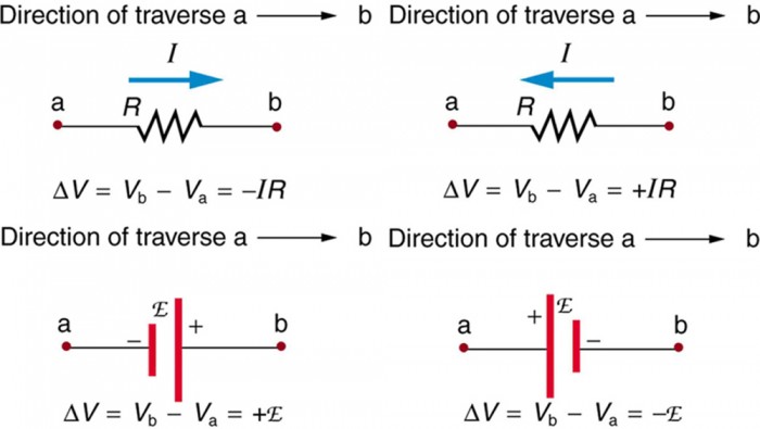
Source: Lumen learning, SUNY physics
To apply Kirchhoff's second rule, the sign of $\Delta V$ is significant: due to the conventions for current, we consider $\Delta V = -IR$ in the case that we measure the potential difference in the same direction as the current and $\Delta V = IR$ in the case that we measure the potential in the opposite direction as the current. The same convention goes for capacitors: $\Delta V = -\dfrac{Q}{C}$ when we measure potential difference in the same direction as the current and $\Delta V = \dfrac{Q}{C}$ when we measure the potential difference in the opposite direction as the current. For EMF sources such as a battery, the sign convention is reversed; we have $\Delta V = \mathcal{E}$ when we measure potential difference in the same direction as the current and $\Delta V = -\mathcal{E}$ when we measure potential difference in the opposite direction as the current. As a summary:
- When measuring in the same direction as the current, then the potential difference across:
- EMF sources are positive
- Resistors are negative
- Capacitors are negative
- When measuring in the opposite direction as the current, then the potential difference across:
- EMF sources are negative
- Resistors are positive
- Capacitors are positive
A perhaps helpful intuitive picture is that current is like a river, an EMF source is like a water pump, a resistor is a place where the river narrows, and a capacitor is like a dam. The pump brings the water (charges) to a higher potential, so it is a positive potential difference, i.e. voltage rise. A narrow part of the river (resistor) dissipates energy from the river (circuit) by slowing it down, so it is a negative potential difference i.e. voltage drop. A dam (capacitor) uses the water to extract useful power, meaning the river downstream (remaining circuit) will flow more slowly, so it is also a negative potential difference. However, this is when we are calculating in the downstream direction (measuring in the same direction as current); if you calculate in the upstream direction, everything will be reversed.
Addendum: Ammeters and voltmeters
Ammeters and voltmeters are different scientific instruments used in electrical circuits. They have important distinguishing features:
- Ammeters are designed to measure current, are connected in series with the circuit, and have minimal resistance. Therefore, by Ohm's law, the current across an ammeter is equal to the current in the circuit, and the voltage across an (ideal) ammeter is zero.
- Voltmeters are designed to measure voltage (potential difference), are connected in parallel with the circuit, and have a high (or at least nonzero) resistance. This means that (ideally) they draw as little current as possible, since parallel circuits divide current across branches but have the same potential difference, so since $I = \dfrac{\Delta V}{R}$, a high resistance means that they draw very little current and don't affect the circuit (much). They internally consist of a joined resistor and ammeter, and therefore, by $\Delta V = I R$ where $I$ is found by the interior ammeter and $R$ is the resistance of the interior resistor, they can calculate and display the voltage.
Magnetic forces and fields
We observe, in nature, that in addition to electric forces, moving charges also generate a magnetic force. The magnetic force on a charge $q$ moving at velocity $\mathbf{v}$ in a magnetic field $\mathbf{B}$ may be defined as:
$$ \mathbf{F} = q\mathbf{v} \times \mathbf{B} $$
Where $\mathbf{B}$ is the magnetic field defined in the SI unit Tesla, denoted $\pu{T}$, where $\pu{1 T = NsC^{-1} * m^{-1}}$. Note that the magnetic force is defined in terms of a cross product, which means that the magnetic force is always perpendicular to the charge's direction of motion. In addition, it may be surprising to find that magnetic forces are velocity-independent - a magnetic force only exists on a moving charge, a charge at rest in a magnetic field does not experience any magnetic force.
One easy source of confusion is that the direction of the force is not the direction the charge moves in. The direction of the force is simply the direction of the acceleration, which is always perpendicular to the charge's direction of motion.
We may find that, surprisingly, that the work done by the magnetic field is zero. This means that the magnetic field cannot impart energy onto the charge, and cannot change the kinetic energy of the moving charge; thus it cannot, on its own, cause a charge to speed up or slow down. It is only electric fields (which are also produced by the charge) that can actually do work and speed up (or slow down) a charge.
$$ W = \int \mathbf{F} \cdot d\mathbf{r} = q\int (\mathbf{v} \times \mathbf{B}) \cdot \mathbf{v} dt = 0 $$
Here in the line integral, we note that $d\mathbf{r} = \mathbf{v} dt$, and since the cross product means that the magnetic force is perpendicular to the velocity vector, its dot product with the velocity vector becomes zero.
Because it is difficult to draw 3D diagrams on 2D paper, we typically represent the direction of the magnetic field with circled crosses and dots, that look like this:

Sourced from Varsity Tutors, "Right Hand Rule For Charge In A Magnetic Field"
The circled dot, on the left, represents a magnetic force pointing out of the page, and the circled dot with a cross, on the right, represents a magnetic force pointing into the page. A good mnemonic is to think of these as arrows for the force vectors; the circled dot is like an arrowhead coming in your direction and the crossed dot is like the tail of the arrowhead moving away from you.
Consider, for instance, an electron moving in a constant magnetic field directed out of the page. Due to the symmetries of the problem, the electron would have a magnetic force that is directed about a fixed center of rotation. This force is a centripetal force that causes the electron to "orbit" the center of rotation.
$$ \mathbf{F} = q\mathbf{v} \times \mathbf{B} = -\dfrac{mv^2}{R} \hat r $$
Therefore, we can rearrange and write it in terms of the magnitudes as:
$$ R = \dfrac{m\|v\|}{q\|B\|} $$
Consider, now, a current through a length of wire, pointing in a certain direction, that can be split into a segment $d\vec\ell$. Recalling that $I = \dfrac{dQ}{dt}$ and $d\vec\ell = \mathbf{v} dt$, we have:
$$ \mathbf{F} = q\mathbf{v} \times \mathbf{B} = \int I dt (\mathbf{v} \times \mathbf{B}) = \int I d \ell \times \mathbf{B} $$
In the case that the wire is a straight line then this simply becomes $\mathbf{F} = I \vec{\ell} \times \mathbf{B}$.
Now consider a magnetic field passing through a loop of current of area $A$ whose normal vector is given by $\hat A$. If the magnetic field lines are uniform and straight, then there is no magnetic force, in accordance with $\mathbf{F} = I \vec\ell \times \mathbf{B}$. If the magnetic field lines are curved, however, there is a net force in the direction the field spreads outwards. We may describe this effect by a quantity known as the magnetic moment $\vec \mu_m = I \vec A$, or for $N$ connected loops, $\vec \mu_m = NI \vec A$. Therefore we have:
$$ \mathbf{F} = \nabla(\vec \mu_m \cdot \mathbf{B}) $$
A coil in a uniform field, however, has no net force, but can have torque, defined as $\vec \tau = \vec \mu \times \mathbf{B}$. Thus, the magnetic field can store potential energy in the coil, and that potential energy is given by $U = -\vec \mu \cdot \mathbf{B}$.
This may seem confusing, because we just said that magnetic forces do no work. We will see later that electric fields associated with magnetic fields in fact do do work, and that a magnetic field is almost always accompanied by an electric field.
The Biot-Savart Law
The Biot-Savart Law is the equivalent of Coulomb's law for the magnetic field. In the discrete case of the magnetic field generated by a moving charge $q$, the Biot-Savart Law is given by:
$$ \mathbf{B} = \dfrac{\mu_0}{4\pi} \dfrac{q\mathbf{v} \times (\mathbf{r} - \mathbf{r'})}{r^3} = \dfrac{\mu_0}{4\pi} \dfrac{q\mathbf{v} \times \hat r}{r^2} $$
Where $\mathbf{r} - \mathbf{r'}$ is the vector pointing from the charge that is located at point $\mathbf{r}' = (x', y', z')$ to a point $(x, y, z)$ in space, $\mathbf{v}$ is the velocity vector of the charge, and $\hat r$ is the unit vector of $\mathbf{r} - \mathbf{r}'$. Note that in problems where symmetries are present, it is sometimes useful to write the Biot-Savart law for a single charge in its explicit form in Cartesian coordinates:
$$ \mathbf{B} = \dfrac{\mu_0 qv}{4\pi} \left(\dfrac{(\hat v \times x\, \hat i) + (\hat v \times y\, \hat j) + (\hat v \times z\, \hat k)}{(x^2 + y^2 + z^2)^{3/2}}\right) $$
The integral expression for the magnetic field, generated by a continuous distribution of charges (i.e., a current), is similarly given by:
$$ \mathbf{B} = \dfrac{\mu_0 I}{4\pi} \int \dfrac{d\mathbf{s}' \times (\mathbf{r}-\mathbf{r}')}{|\mathbf{r}-\mathbf{r}'|^3} $$
Where $I$ is the current, $d\mathbf{s}'$ is a segment of the current-carrying wire that is located at $\mathbf{r}'$, and again, $\mathbf{r} - \mathbf{r}'$ is the vector pointing from $d\mathbf{s}'$ to $(x, y, z)$. An illustration is shown below for a more visual explanation of the equation (note, however, that in this illustration, $d\mathbf{s}'$ is written as $d\mathbf{s}$):
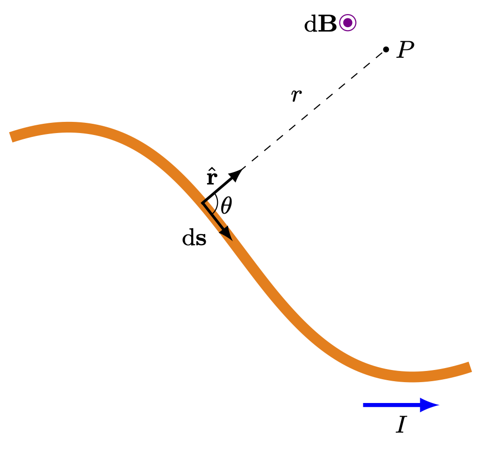
The Biot-Savart law was found experimentally, just like Coulomb's law; however, there are some key differences:
- Magnetic fields only exist when a charge is moving
- The field is perpendicular to the direction of current
- The field lines form closed circles as opposed to outward or inward flowing lines
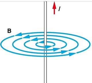
A diagram of magnetic fields, sourced from Physics Stack Exchange
Ampère's law
We may also calculate the magnetic field through Ampère's law. Ampère's law equates the line integral of the magnetic field through a loop with the enclosed current flowing through the cross-section formed by the loop:
$$ \oint \limits_\mathrm{loop} \mathbf{B} \cdot d\mathbf{r} = \mu_0 I_\mathrm{enc.} $$
Where $\mu_0 \approx 4\pi \times 10^{-7}$ is the magnetic constant and $I_\mathrm{enc.}$ is the enclosed current (which may be a function of position). There are also alternative formulations of Ampère's law, which are completely equivalent. For instance, there are cases in which it is helpful to write Ampère's law in terms of the current density, in the following form:
$$ \oint \limits_\mathrm{loop} \mathbf{B} \cdot d\mathbf{r} = \mu_0 \iint \mathbf{J} \cdot d\mathbf{A} $$
Which, in the particular case that the current flows across a circular cross-sectional area of radius $r$, reduces to:
$$ \oint \limits_\mathrm{loop} \mathbf{B} \cdot d\mathbf{r} = \mu_0 \int_0^r J(r')2\pi r', dr' $$
Ampère's law applies in only certain conditions. First, the loop must be around a closed loop. Second, the loop must be around the edges of a cross section where current is flowing through.
The diagram below demonstrates the correct application of Ampère's law. We have a cross section $S$ that has current $I_\mathrm{enc}$ passing through. The magnetic field $\mathbf{B} = B \hat \theta$ flows in a circle around the current-carrying wire. Thus, the line integral would be integrating over the boundary of $S$, which forms a closed loop.
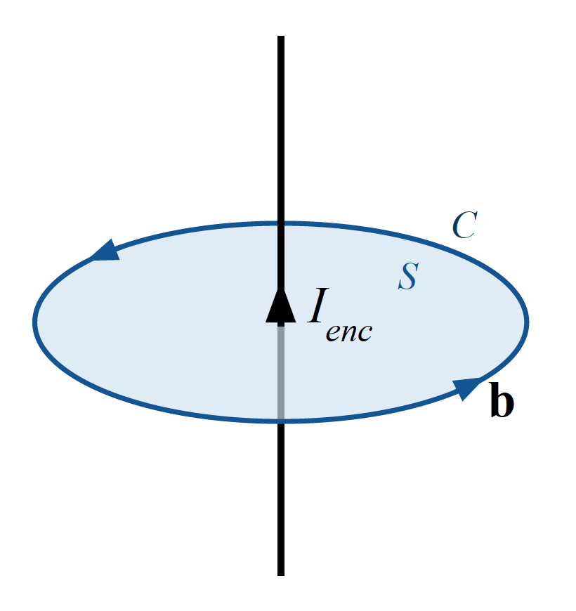
An analytical solution to Ampère's law may be found when the correct loop is chosen such that the magnetic field is uniform along the loop. For instance, in the case of an infinitely long current-carrying wire, Ampère's law becomes:
$$ \oint \mathbf{B} \cdot d\mathbf{r} = B(2\pi r) = \mu_0 I $$
Thus the magnetic field is given by:
$$ |\mathbf{B}| = \dfrac{\mu_0 I}{2\pi r} $$
We may also consider the case of a solenoid, which is a long coil of wire that forms an electromagnet of length $L$. If we consider a rectangular loop that goes into and out of the coil, we find that Ampère's law reduces to:
$$ \oint \mathbf{B} \cdot d\mathbf{r} = BL = \mu_0 I_\mathrm{enc.} = \mu_0 N I $$
Where $N$ is the total number of connected coils and $I$ is the current in each coil. We may rearrange to obtain the magnetic field of a solenoid:
$$ \mathbf{B} = \mu_0 \dfrac{NI}{L} \hat{\mathbf{x}} $$
Remember that akin to Gauss's law, a net zero enclosed current does not imply that the magnetic field has to be zero everywhere, or that there are no currents within a region. It may simply be the case that there are currents and fields that cancel each other out. Also recall that just like Gauss's law, any magnetic fields outside the loop have no effect on the magnetic field within the loop; conversely Ampère's law only gives the magnetic field within the loop and says nothing about what is outside.
Faraday's law and electromagnetic induction
We observe that a changing magnetic flux through a given non-closed surface produces an electric field that circulates around the boundary of the surface. A classic example is moving a magnet through a series of coils (or moving a coil through the magnetic field of a magnet). This phenomenon is known as electromagnetic induction because electric fields are induced by changing magnetic flux. This is is Faraday's Law:
$$ \int_C \mathbf{E} \cdot d \mathbf{r} = -\dfrac{d}{dt}\iint \mathbf{B} \cdot d\mathbf{A} $$
Faraday's law can also be expressed in any of the following ways:
$$ \int_C \mathbf{E} \cdot d \mathbf{r} = -\dfrac{d\Phi_B}{dt} = -\dfrac{d}{dt}\iint \mathbf{B} \cdot d\mathbf{A} = \mathcal{E}_\mathrm{loop} $$
Note of caution: here, the sign convention is used that positive flux flows out of surface and negative flux enters a surface, where the surface's orientation is defined by the direction of its normal vector. We also use the convention that the surface normal for the area element is the cross product $\hat n = \hat e_1 \times \hat e_2$ where $e_1, e_2$ are the coordinate unit vectors on the surface. For a plane aligned on the XY plane, this would be $\hat n = \hat x \times \hat y$. For any questions that showcase a 2D loop, assume the normals are pointing out of the page unless otherwise stated.
Calculating magnetic flux
The process of calculating magnetic flux can be tricky, so let us consider an example to demonstrate the calculation process. Consider a very long wire carrying current $I$ in the rightward direction, with a wire loop of width $w$ and height $b-a$ below it, as shown in the diagram below:

We note that the magnetic field vectors go into the page while the wire loop's normal points out of the page, meaning they are antiparallel (parallel but pointing in opposite directions). Therefore, we know that $\mathbf{B}(r) \cdot d\mathbf{A} = -B(r) dA$ where $dA = dr dx$ is the area of an infinitesimal portion of the loop's surface. Now, recalling that $B = \dfrac{\mu_0 I}{2\pi r}$ for a current-carrying wire of infinite (or at least very long) length, which we derived earlier from Ampère's law, if we substitute our derived expressions into the integral equation for the magnetic flux, we have:
$$ \begin{align*} \Phi_B &= \iint \limits_\mathrm{surface} \mathbf{B} \cdot d\mathbf{A} \\ &= -\int_0^w \int_a^{a+b} \dfrac{\mu_0 I}{2\pi r} \, dr\, dx \\ &= \int_0^w\left(-\dfrac{\mu_0 I}{2\pi}\right) \int_a^{a+b} \dfrac{1}{r} dr\, dx \\ &= \int_0^w \dfrac{\mu_0 I}{2\pi} \int_{a+b}^a \dfrac{1}{r} dr\, dx \\ &= \dfrac{\mu_0 I}{2\pi} \int_0^w \ln(r) \bigg|_{a+b}^a dx \\ &= \dfrac{\mu_0 I}{2\pi} \int_0^w (\ln(a) - \ln(a+b)) dx \\ &= \dfrac{\mu_0 I}{2\pi} \int_0^w \ln\left(\dfrac{a}{a+b}\right) dx\\ &= \dfrac{\mu_0 I w}{2\pi}\ln\left(\dfrac{a}{a+b}\right) \end{align*} $$
Sources of changing magnetic flux
Faraday's law only applies when magnetic flux is changing with time. There are three main ways this may occur:
- The magnetic field itself is changing. This is the case with a non-constant magnetic field, such as those produced by changing currents, or oscillating magnetic fields in free space (which we'll see more on later)
- The area of the surface through which the flux is measured is changing. This is the case when a wire loop, for instance, is pulled into or out of a region of constant magnetic field; the area of the loop exposed to the field changes, causing a change in flux
- The angle between the magnetic field and the surface's normals is changing. This is the case when we have a rotating wire loop; since flux is dependent on the angle between the surface normals and the magnetic field, a rotating wire loop causes a nonzero magnetic flux
Sign of Faraday's Law and Lenz's Law
The negative sign on the right-hand side of Faraday's law is due to the fact that the the induced electric field, and $\mathcal{E}$ is known as the EMF (confusingly named the electromotive force) which is a potential difference. And we know from $\mathbf{E} = -\nabla V$ that a potential difference causes an electric field to flow between the points of differing potential. This electric field, however, is non-conservative and unlike electrostatic fields, this electric field always forms a closed loop.
The negative sign is in fact quite significant. We use it to define Lenz's law:
$$ \mathcal{E}_\mathrm{loop} = -\dfrac{d\Phi_B}{dt} $$
And the average EMF as:
$$ \mathcal{E}_\mathrm{avg} = -\dfrac{\Delta \Phi}{\Delta t} $$
Lenz's law is significant because it shows that the current produced by a changing magnetic flux is opposed to the change in flux. This is because the induced current generates another magnetic field that opposes the external magnetic field by $\mathbf{F} = I\vec \ell \times \mathbf{B}_\mathrm{generated}$. In other words, an increasing flux creates a negative current; a decreasing flux creates a positive current. In each case, the induced current produces a magnetic field that opposes the external magnetic field and thus the change in flux.
Note on sign: a positive current is (by convention) one that flows counterclockwise. A negative current is one that flows clockwise. Thus positive flux creates clockwise current and negative flux creates counterclockwise current. In both cases, the current direction is opposite to the current in the loop, and the direction of the current will tell us the induced force on the wire without even needing to calculate the flux.
We showcase Lenz's law in the diagram below:

If a changing flux occurs as a result of the motion of a conducting surface or loop, we call the resulting EMF motional EMF. Lenz's law tells us that a given loop of wire (or any other general conductor) moving at velocity $\mathbf{v}$, then the direction of the net force on the loop/conductor by Lenz's law is opposite the direction of $\mathbf{v}$. This also means there is no force when $\mathbf{v} = 0$ because the magnetic flux is constant in time (it may vary spatially but would not vary in time).
When the induced electric field around the boundary of a loop happens to be in a wire, then we find that the EMF creates a current given by Ohm's law:
$$ I = \dfrac{\mathcal{E}}{R} $$
Aside: The unit of magnetic flux is called the Weber $\pu{Wb}$, where $\pu{1Wb} = \pu{1V} \cdot \pu{s}$. The unit of the EMF is the same as potential difference, i.e. the EMF is in units of $\pu{V}$ (volts).
Displacement current
We now need to return to Ampère's law. Recall that the previous formulation of Ampère's law was valid for the electrostatic case, and was given by:
$$ \oint \limits_\mathrm{loop} \mathbf{B} \cdot d\mathrm{r} = \mu_0 I_\mathrm{enclosed} = \mu_0 \iint \mathbf{J} \cdot d\mathbf{A}_\text{cross section} $$
However, now with the knowledge that changing magnetic flux induces an electric field, we find that there is a contradiction. The current passing through a loop around a magnetic field is not simply the current passing through the cross-sectional area bounded by the loop. There is also an induced current produced by the changing flux of the magntic field through the cross-section area. Therefore, scientist James Clerk Maxwell postulated that a changing electric flux $\dfrac{d\Phi_E}{dt}$ through a non-closed surface also induces a magnetic field:
$$ \oint \limits_\mathrm{loop} \mathbf{B} \cdot d\mathrm{r} = \mu_0 I_\mathrm{enc.} + \mu_0 \epsilon_0 \dfrac{d}{dt}\iint \mathbf{E} \cdot d\mathbf{A} $$
This additional term is known as the displacement current and completes Ampère's law by accounting for the interplay between electric and magnetic fields. With this, the four Maxwell equations are complete.
Inductors
We recall that Faraday's law says that an EMF is generated with a time-varying magnetic flux across an open surface. We also recall from Lenz's law that this produces an electric field whose field lines form a closed loop about the boundary of the surface, creating a current opposed to the change in magnetic flux.
Inductors are electrical devices that use the principle of electromagnetic induction to oppose the change in current, but unlike resistors that dissipate the energy away as waste heat, inductors store the energy within a magnetic field and slowly release it back into the circuit. We measure this property of an inductor with a quantity known as the inductance $L$ given in the unit $\pu{H}$ (henry), that describes the induced current as proportional to the flux with the constant factor $L$. There are two types of inductance:
- Self-inductance: inductance $L$ caused by the flux of one conductor acting on itself, resulting in an induced current: $L = \dfrac{\Phi_B}{I}$ for a single coil or $L = \dfrac{N\Phi_B}{I}$ for a coil with $N$ loops/turns
- Mutual inductance: inductance $M$ caused by the flux of one conductor (coil 1) acting on another conductor (coil 2): $M = \dfrac{\Phi_\text{induced in 2}}{I_1}$ for a single coil or $M = \dfrac{N_2\Phi_\text{induced in 2}}{I_1}$ for coil 2 with $N_2$ turns
The inductance has several important properties:
- It is independent of current, only depending on the geometry of the conductors/inductors. This means for a given material within the same conditions (pressure, composition, temperature, etc.) it is a constant
- The mutual inductance is also independent of the conductor you establish as creating the flux and the conductor you establish as having an inducted current. That is to say, $M = \dfrac{N_2\Phi_\text{induced in 2}}{I_1} = \dfrac{N_1 \Phi_\text{induced in 1}}{I_2}$, where $\Phi_\text{induced in 1}$ is the flux induced in coil 1, $\Phi_\text{induced in 2}$ is the flux induced in coil 2, $I_1$ is the current in coil 1, $I_2$ is the current in coil 2, and $N_1, N_2$ are the respective number of coils in coil 1 and 2
Consider, for instance, a solenoid with $N$ turns and magnetic field $\mathbf{B} = \mu_0 n I \hat{\mathbf{x}}$ where $n = N/\ell$ is the number of turns per unit length. The flux through a cross-section of the solenoid would be given by $\Phi_B = B A = \mu_0 n I A = \mu_0 n I \pi R^2$. The (self-)inductance would be $L = \dfrac{\Phi_B}{I} = \mu_0 n^2 \pi R^2$.
When we take the time derivative of the flux, we note that since $L$ is a constant, we have:
$$ \dfrac{d\Phi_B}{dt} = L \dfrac{dI}{dt} $$
Which we may rewrite as:
$$ \mathcal{E} = -L \dfrac{dI}{dt} $$
Upon examination, we see a quantity that is an EMF that is related to the inductance - the back EMF. We will examine its significance in the following section.
Back EMF
The relationship $\mathcal{E} = -L \dfrac{dI}{dt}$ tells us that a change in current produces a back EMF that is opposed to the change in current, because of the negative sign. This back EMF is dependent on the rate of change of a current, so a rapid change in current will result in a back EMF in the opposite direction as the current, reducing the current significantly. This property is very useful in many cases, and is why inductors are often used as surge protectors in circuits and for protection against lightning strikes.
In addition, since the back EMF is opposed to the current, we have $-\Delta V = L \dfrac{dI}{dt} = V(a) - V(b)$ where $V(a)$ is the potential on the inside of the inductor and $V(b)$ is the potential on the outside of the inductor. The induced electric field caused by this potential difference $\mathbf{E}\mathrm{induced} = -\nabla V$ counters the electrostatic field inside the inductor due to its own charge, meaning that the total electric field $\mathbf{E}\mathrm{net} = 0$, as we would expect because a conductor must have zero net electric field.
Inductors as circuit components
The potential induced by a conductor attempts to maintain the current and acts as a voltage drop in the circuit proportional and opposite to the change in current. Therefore, aligning our circuit direction such that it is between points $a$ and $b$ where current flows from $a \to b$, the inductance behaves in one of three ways:
- If the current stays constant, the inductor has no effect
- If the current increases, the inductor produces a negative back EMF and thus acts as a voltage drop in the direction of the current that slows the change in current
- If the current decreases, the inductor still produces a negative back EMF in the direction of the current and thus still acts as a voltage drop
- Total inductance fo llows $L_P = \left(\dfrac{1}{L_1} + \dfrac{1}{L_2} + \dfrac{1}{L_3} + \dots + \dfrac{1}{L_n}\right)^{-1}$ for parallel circuits and $L_S = L_1 + L_2 + L_3 + \dots + L_n$ for series circuits
Inductors and magnetic energy
We have seen that static magnetic fields cannot do work (and thus has no defined potential energy in the conventional sense), but this does not mean they cannot store energy. Recall that we may write the magnetic energy as the time integral of the power, from which we may rearrange to find an expression of energy stored in the field:
$$ U_B = \int P(t) \,dt = \int I \mathcal E dt = \int I L \dfrac{dI}{dt}\, dt = \dfrac{1}{2} LI^2 $$
We may find the specific case of the energy stored in the the time-varying magnetic field as:
$$ U_B = \dfrac{1}{2} L I^2 = \dfrac{1}{2} \mu_0 n^2 \pi R^2 I^2 $$
But since we know that $B = \mu_0 n I$, and dividing by volume, we have:
$$ u_B = \dfrac{1}{2\mu_0} B^2 $$
This is a general expression that is independent of any circuit, and thus it must be fundamental to electromagetism, beyond just applicable to a specific component. Indeed, later, we show that this is indeed the case.
Transient circuits
We have already seen and calculated some of the quantitative characteristics of different electrical components, such as resistors, capacitors, and inductors. We will now analyze circuits, formed through a series of connected electrical components. By careful application of our previously-derived expressions for the potential difference and EMF of electrical components, we can find how the current, voltage, and charge evolves through time. This is termed the analysis of transient circuits, transient meaning that such circuits are undergoing transitions.
RC circuit
An RC circuit refers to a resistor and a capacitor connected in series to an EMF source (i.e. battery). Recall that we may write $\Delta V = \left|\dfrac{Q}{C}\right|$ for a capacitor and $\Delta V = IR$ for a resistor. By Kirchhoff's rules and the associated sign convention (a resistor is a drop in voltage, a capacitor is also a drop in voltage, so both are negative in sign) we have:
$$ \sum_i \Delta V_i = \mathcal{E} -\dfrac{Q}{C} - IR = 0 $$
Now rewriting $I = \dfrac{dQ}{dt}$ we find a differential equation:
$$ \mathcal{E} - \dfrac{Q}{C} - R\dfrac{dQ}{dt} = 0 $$
We may rearrange to write it in more conventional form as:
$$ \dfrac{dQ}{dt} = \dfrac{\mathcal{E}}{R} - \dfrac{Q}{RC} $$
This differential equation may be solved by the method of the separation of variables. The general solution of the differential equation can then be used to find two important particular solutions for different initial conditions of $Q$. In addition, we may further differentiate the solutions for the charge $Q(t)$ to find the current, and use $V = Q/C$ to find the voltage (note: $V$ is a shorthand for $\Delta V$ here). The results are shown in the table below:
| Initial condition | Solution | Solution description |
|---|---|---|
| $Q(0) = 0$ | $Q(t) = \mathcal{E} C(1 - e^{-t/RC}) = Q_\mathrm{max},(1 - e^{-t/\tau})$ | Uncharged open circuit with switch closed at $t = 0$, causing the circuit to start charging. |
| $Q(0) = \mathcal{E}C = Q_\mathrm{max}$ | $Q(t) = \mathcal{E} Ce^{-t/RC} = Q_\mathrm{max},e^{-t/\tau}$ | Fully-charged closed circuit with switch opened at $t = 0$, causing the circuit to start discharging. |
| $I(0) = I_0 = \dfrac{\mathcal{E}}{R}$ | $I(t) = \dfrac{\mathcal{E}}{R} e^{-t/RC} = I_0 e^{-t/\tau}$ | Charging case, where $Q(0) = 0$ |
| $I(0) = 0$ | $I(t) = \dfrac{\mathcal{E}}{R} (1 - e^{-t/RC}) = I_\mathrm{max} (1 - e^{-t/\tau}), I_\mathrm{max} = \dfrac{\mathcal{E}}{R}$ | Discharging case, where $Q(0) = Q_\mathrm{max}$ |
| $V(0) = 0$ | $V(t) = \mathcal{E}(1 - e^{-t/RC}) = V_\mathrm{max} (1 - e^{-t/\tau})$ | Charging case, where $Q(0) = 0$ |
| $V(0) = V_0 = \mathcal{E}$ | $V(t) = \mathcal{E} e^{-t/RC} = V_0 e^{-t/\tau}$ | Discharging case, where $Q(0) = Q_\mathrm{max}$ |
Note: Be careful of the interpretations of $I, Q, V$. $I$ is the current through the series circuit (which is identical at the resistor and the capacitor as all components are connected in series). By contrast, $V$ is the potential difference at the resistor and $Q$ is the charge stored in the capacitor. Saying simply "charge" or "voltage" can easily be misleading as these are not applicable to each component.
Note that $\tau = RC$ is the time constant, a period-like quantity that measures how much the circuit is charged (for case 1, i.e. $Q(0) = 0$) or how fully the circuit has discharged (for case 2, i.e. $Q(0) = Q_\mathrm{max}$). The specific values of the time constant are related to the charge as follows:
| Time constant | Percent charge relative to $Q_\mathrm{max}$ (in charging case) | Percent charge relative to $Q_\mathrm{max}$ (in discharging case) |
|---|---|---|
| $t = 0$ | 0.0% | 100.0% |
| $t = \tau$ | 63.2% | 36.8% |
| $t = 2\tau$ | 86.5% | 13.5% |
| $t = 3\tau$ | 95.0% | 5.0% |
| $t = 4\tau$ | 98.2% | 1.8% |
| $t = 5\tau$ | 99.3% | 0.7% |
| $t = 6\tau$ | 99.8% | 0.2% |
We see that the current in the circuit and potential difference across the resistor increase as the capacitor charges, and decrease as the capacitor discharges. The current behaves the opposite way, as it decreases to as the capacitor charges and increases as the capacitor discharges. This can be intuitively thought of as the charging capacitor "holding" more and more charge until it reaches its maximum charge and no more charge can flow in, meaning the current (which is the flow of charge) becomes zero. The opposite cocurs as the capacitor discharges since the capacitor "releases" more and more charge until it holds no charge, meaning the charges flow out and the current increases until no more charge can flow out of the capacitor, at which point the current has reached its maximum.
RL circuit
We will now discuss the first of two circuit types that involve an inductor - RL circuits and LC circuits. In the first, let us consider an RL circuit: a circuit with an EMF source that provides an EMF $\mathcal{E}$ attached to a resistor and an inductor, hence the name (given that $L$ is the symbol for inductance). Then by Kirchhoff's loop rule, recalling that both resistors and inductors are voltage drops, we have:
$$ \mathcal{E} - IR - L \dfrac{dI}{dt} = 0 $$
This is a differential equation that can be solved for the current $I$, using the typical methods for differential equations, such that for the initial conditions $I(0) = 0$ (that is, the circuit is closed at $t = 0$, allowing current to flow), we have:
$$ \begin{matrix} I(t) = I_\mathrm{max} (1 - e^{-t/\tau}), & I_\mathrm{max} = \dfrac{\mathcal{E}}{R} \\ V_L(t) = -L \dfrac{dI}{dt} = -\mathcal{E} e^{-t/\tau}, &\tau = L/R \end{matrix} $$
Note: $V_L$ is the potential difference across the inductor, not at every point in the circuit!
LC circuit
Finally, we examine LC circuits, which are composed of an inductor and a capacitor. Given that a capacitor stores charge where $Q = CV$, and assuming that the capacitor has nonzero charge at $t= 0$, we can use Kirchhoff's loop rule again to have:
$$ -\dfrac{Q}{C} - L \dfrac{dI}{dt} = 0 $$
Or if we multiply all sides by $-1$ to clean up the equation:
$$ \dfrac{Q}{C} + L \dfrac{dI}{dt} = 0 $$
But recall that current is the time derivative of charge, so we may equivalently write $\dfrac{dI}{dt} = \dfrac{d^2 Q}{dt^2}$ and the differential equation becomes:
$$ \begin{gather*} \dfrac{Q}{C} + L \dfrac{d^2Q}{dt^2} = 0 \\ \dfrac{d^2Q}{dt^2} + \dfrac{1}{LC} Q(t) = 0 \end{gather*} $$
If we define a quantity $\omega_0$ called the resonant frequency where $\omega_0 = \dfrac{1}{\sqrt{RC}}$ this may be equivalently written as:
$$ \dfrac{d^2Q}{dt^2} + \omega_0^2 Q(t) = 0 $$
Again, by using the typical methods of solving 2nd-order linear differential equations and assuming that the circuit starts off with 100% of the charge on the capacitor we obtain the solution:
$$ Q(t) = Q_\mathrm{max} \cos (\omega_0 t + \phi) $$
Where $Q(t)$ is the charge on the capacitor - which is oscillating sinusoidally in time, and $\phi$ is a delay factor of the sinusoid, representing a time shift. The corresponding voltage on the inductor is given by:
$$ \begin{matrix} V(t) = V_0 \cos (\omega_0 t + \phi), &V_0 = LQ_0 \omega_0^2 \end{matrix} $$
AC circuits and phasors
When considering AC circuits, we find that we encounter harmonic functions that vary non-trivially with time for the vast majority of quantities. While we can use sines and cosines to describe harmonic functions, it is more convenient, and indeed sometimes simply more useful, to use complex exponentials.
This is possible through Euler's formula $e^{j\phi} = \cos \phi + j \sin \phi$ (and the related identity $e^{-j\phi} = \cos \phi - j \sin \phi$). Thus, we may write the voltage $V(t) = V_0 \cos (\omega t)$ as $V(t) = V_0 e^{j\omega t}$ in phasor form. Using the rules of exponential multiplication and division makes it far easier to work with phasors, and we can always use Euler's formula to extract the real part of the phasor.
Note on notation: Here $j$ is the same as the imaginary unit $i$, the only reason why $j$ is the preferred symbol over $i$ is that it is less likely to be confused with the current, which also has symbol $i$.
Consider an AC circuit with a resistor, which has a source of variable EMF $V(t) = V_0 e^{j \omega t}$. With Ohm's law, $I_0 = V_0 / R$, we find that $I(t) = I_0 e^{j \omega t}$. This is a very interesting relationship, as it shows that potential difference and current in an AC circuit are always in phase for a resistor.
This is not necessarily always the case for other electrical components. For instance, a capacitor has $Q = CV$, and thus $Q(t) = C V_0 e^{j \omega t}$. Taking the derivative, we have $I(t) = \dfrac{dQ(t)}{dt} = C V_0 j \omega e^{j \omega t}$, where multiplication by $j$ is equivalent to a 90-degree rotation in the complex plane, i.e. $j = e^{j\pi/2}$. Thus, we may equivalently write $I(t) = CV_0 \omega e^{j (\omega t + \pi/2)}$. That is to say, in capacitors, the phase of the current leads (is ahead of) the phase of the voltage by $\pi/2$.
In AC circuits both capacitors and inductors have a form of resistance in addition to resistors, which we call the reactance with symbol $X$. For resistors, $X_R = R$ and so its reactance is just the normal resistance, but for capacitors $X_C = \dfrac{1}{\omega C}$ and for inductors $X_L = \omega L$. Ohm's law, which we previously introduced as $V = IR$, becomes modified to $V = I X$. With these definitions, we may write our previous expression for the current passing through a capacitor $I(t) = CV_0 \omega e^{j (\omega t + \pi/2)}$ as $I(t) = \dfrac{V_0}{X_C} e^{j(\omega t + \pi/2)}$. Since $V = IX$ and thus $V_0 = I_0 X_C$ we can also write this as $I(t) = I_0 e^{j(\omega t + \pi/2)}$. This is perhaps the most simplified and easily-understandable form of the current through a capacitor. We may do the same for inductors to determine the current and voltage through an inductor
In an alternating circuit, described by phasors, the reactance forms the imaginary part of a complex number called the impedance, denoted $Z$, whose real part is the resistance $R$. Therefore, we have:
$$ Z = R + j X $$
Thus, the most general form of Ohm's law, as applicable to AC circuits, is given by $V = IZ$, and if we substitute the values we found for the reactance into the formula for the impednace, we find the following:
| Component | Impedance | Current vs. Voltage Phase Shift |
|---|---|---|
| Resistor | $R$ | Always in phase |
| Capacitor | $\dfrac{1}{j\omega C}$ | Current leads voltage by $\pi/2$ |
| Inductor | $j\omega L$ | Current lags voltage by $\pi/2$ |
The Maxwell equations
We have now reached the culminating point of classical electromagnetism. Recall that electromagnetism is a classical field theory, where knowing the fields is sufficient to uniquely determine the motion of every charge within the fields (which is also every charge creating the field). The equations that govern how electromagnetic fields (the electric field $\mathbf{E}$ and the magnetic field $\mathbf{B}$) are the Maxwell equations, and here is a brief description of each:
$$ \oiint \limits_\mathrm{surface} \mathbf{E} \cdot d\mathbf{A} = \dfrac{Q_\mathrm{enc.}}{\epsilon_0} = \dfrac{1}{\epsilon_0} \iiint \limits_\mathrm{volume} \rho\, dV $$
The first of Maxwell's equations, shown above, is Gauss's law for electric fields. Its physical interpretation is that an imaginary closed surface was placed in space, the total flux (outward flow) of the electric field across the surface would be proportional to the total enclosed electric charge.
$$ \oiint \limits_\mathrm{surface} \mathbf{B} \cdot d\mathbf{A} = 0 $$
The second of Maxwell's equations, shown above, is Gauss's law for magnetic fields. Its physical interpretation is that if an imaginary closed surface was placed in space, the total flux (outward flow) of the magnetic field across the surface is zero, because ingoing and outgoing field lines cancel out. Thus, there exist no magnetic monopoles (pure sources).
$$ \oint \limits_\mathrm{loop} \mathbf{E} \cdot d\ell = -\dfrac{\partial}{\partial t} \iint \limits_\mathrm{surface} \mathbf{B} \cdot d\mathbf{A} $$
The third of Maxwell's equations, shown above, is Faraday's law. Its physical interpretation is that if an imaginary surface (that is not closed) was placed in space, the change in flux of the magnetic field across the surface induces an EMF and therefore an electric field that circulates in a loop across the boundary of the surface. By Ohm's law, this results in a current if the loop is a wire or conductor. Faraday's law predicts that a magnetic field whose field lines form closed loops is always found alongside an electric field.
$$ \oint \limits_\mathrm{loop} \mathbf{B} \cdot d\ell = \mu_0 I + \mu_0 \epsilon_0 \dfrac{\partial}{\partial t} \iint \limits_\mathrm{surface} \mathbf{E} \cdot d\mathbf{A} $$
Finally, the fourth of Maxwell's equations, shown above, is the Maxwell-Ampère law. If an imaginary surface (not closed) were placed in space, the change in flux of the electric field across the surface induces a magnetic field that circulates in a loop across the boundary of the surface. The Maxwell-Ampère law predicts that a magnetic field whose field lines form closed loops is always found alongside an electric field.
Recall the divergence theorem from vector calculus, which relates the surface integral of a vector field $\mathbf{F}$ over a closed surface to the volume integral of the divergence of $\mathbf{F}$ across the volume bounded by the surface:
$$ \oiint_{\partial \Omega} \mathbf{F} \cdot d\mathbf{A} = \iiint_\Omega \nabla \cdot \mathbf{F}\, dV $$
In addition, Stoke's theorem from vector calculus relates the line integral of a vector field $\mathbf{F}$ around a closed loop to the surface integral of its curl across the cross-section formed by the loop:
$$ \oint_{\partial S} \mathbf{F} \cdot d\mathbf{r} = \oiint_S \nabla \times \mathbf{F} \cdot d\mathbf{A} $$
From here, we can convert the integral equations into differential equations that are the most common formulation of Maxwell's equations:
$$ \begin{align*} \nabla \cdot \mathbf{E} &= \dfrac{\rho}{\epsilon_0} \\ \nabla \cdot \mathbf{B} &= 0 \\ \nabla \times \mathbf{E} &= -\dfrac{\partial \mathbf{B}}{\partial t} \\ \nabla \times \mathbf{B} &= \mu_0 \mathbf{J} + \mu_0 \epsilon_0 \dfrac{\partial \mathbf{E}}{\partial t} \end{align*} $$
From the differential equation form (also called the differential form), the physical interpretation of Maxwell's equations becomes more streamlined. The first two equations show that electric fields are produced by ("flow out of") a diverging charge density $\rho$, and that magnetic fields have zero divergence, as they flow from a north to south pole in closed field lines. The last two equations show that time-varying magnetic fields produce electric fields that curl around the magnetic fields, and that time-varying electric fields produce magnetic fields that curl around the electric fields.
The Maxwell equations are astoundingly universal in scope. They govern electromagnetic interactions down to the atomic level, and only at the subatomic level are quantum descriptions necessary. They are truly one of the most beautiful and successful equations in physics.
Electromagnetic waves
Among the most famous theoretical predictions of Maxwell's equations is that in the absence of sources, i.e. when $\nabla \cdot \mathbf{E} = 0, \nabla \cdot \mathbf{B} = 0$, the electric field and magnetic field obey a wave equation:
$$ \begin{align*} \dfrac{\partial^2 \mathbf{E}}{\partial t^2} = \mu_0 \epsilon_0 \nabla^2\mathbf{E} \\ \dfrac{\partial^2 \mathbf{B}}{\partial t^2} = \mu_0 \epsilon_0 \nabla^2\mathbf{B} \end{align*} $$
Surprisingly, by comparison with the general form of the wave equation, it can be shown that the velocity of propagation of these waves is a constant, given by $\dfrac{1}{\sqrt{\mu_0 \epsilon_0}}$. This we know more commonly as the speed of light, $c$, meaning that all light is an electromagnetic phenomenon. This fact was empirically verified by Heinrich Hertz, who proved that electric and magnetic fields do indeed create electromagnetic waves that propagate at the speed of light $c$. That is to say, any combination of a time-varying electric field and a time-varying magnetic field produces a self-sustaining and self-propagating electromagnetic wave that travels across space. Among the multiple applications and consequences of this fact is one that is essential in everyday life: Wi-Fi signals are carried by electromagnetic waves, in addition to telecommunications and fiberoptic cables, which is to say that the modern digital world and internet is made possible by our understanding of electromagnetic waves.
The simplest solutions to the electromagnetic wave equations, after applying the suitable boundary conditions (for the curious, they are $\mathbf{E}(\mathbf{r}, 0) = \mathbf{E}_0$, $\mathbf{E}(\mathbf{r}, t) = \mathbf{E}(\mathbf{r}, t + T)$, $\mathbf{E}(\mathbf{r}, t) = \mathbf{E}(\mathbf{r} + \lambda, t)$ where $T$ is the period and $\lambda$ is the wavelength, and analogous for the magnetic field), are given by:
$$ \begin{align*} \mathbf{E}(\mathbf{r}, t) = \mathbf{E}_0 \cos (\mathbf{k} \cdot \mathbf{r} - \omega t) \\ \mathbf{B}(\mathbf{r}, t) = \mathbf{B}_0 \cos (\mathbf{k} \cdot \mathbf{r} - \omega t) \\ \end{align*} $$
These solutions are known as harmonic plane-wave solutions. Here, $\mathbf{E}_0$ is the electric field amplitude and $\mathbf{B}_0$ is the magnetic field amplitude. In addition, $\omega$ is the angular frequency given by $\omega = 2\pi f$ where $f = \dfrac{1}{T}$; meanwhile, $\mathbf{k}$ is known as the wavevector, whose direction is the direction of propagation of the wave and whose magnitude is given by $\dfrac{2\pi}{\lambda}$ where $\lambda$ (as mentioned previously) is the wavelength, and $\lambda = \dfrac{c}{f}$.
Note: plane waves are not physically realistic as they have infinite length and would require an infinite amount of energy to create. They, are, however, a good theoretical approximation. Realistic and physically-allowable waves are actually given by continuous superpositions of plane-wave solutions, and thus we have $\mathbf{E}(\mathbf{r}, t) = \displaystyle \iiint \dfrac{d^3k}{(2\pi)^3}\mathbf{A}(\mathbf{k}) \cos (\mathbf{k} \cdot \mathbf{r} - \omega t)$ and analogous for the magnetic field. In addition, realistic waves are typically semi-spherical in nature due to the conservation of energy.
For plane-wave solutions, it is always the case that $\mathbf{E}_0 \cdot \mathbf{B}_0 = 0$, meaning that the electric and magnetic fields are always perpendicular each other, and $\mathbf{E}_0 \cdot \mathbf{k} = \mathbf{B}_0 \cdot \mathbf{k} = 0$, meaning that the electric and magnetic fields always oscillate transverse (perpendicular to) the direction of propagation of the wave. The electric field amplitude and the magnetic field amplitude are further related by $\mathbf{E}_0 = c \mathbf{B}_0$, in the case of plane waves.
Electromagnetic waves also carry energy and momentum. In fact, energy from the Sun is carried to Earth purely in the form of electromagnetic waves. As it does not make a lot of sense to speak of the total energy of an electromagnetic wave (as the electromagnetic wave is spread over all space instead of having a definite position), we instead describe the energy density (energy per unit volume) of electromagnetic waves. This is more applicable given that energy is transferred through electromagnetic waves between different locations in space. The electrical energy density $u_E$ and magnetic energy density $u_B$ of the electric and magnetic components of an electromagnetic wave are respectively given by:
$$ \begin{matrix*} u_E = \dfrac{1}{2}\epsilon_0 E_0^2, &u_B = \dfrac{1}{2\mu_0}B_0^2 \end{matrix*} $$
Where the electromagnetic energy density is simply their sum:
$$ u = u_E + u_B = \dfrac{1}{2} \epsilon_0 E_0^2 + \dfrac{1}{2\mu_0} B_0^2 $$
The power carried by electromagnetic waves is given by the Poynting vector:
$$ \mathbf{S} = \dfrac{1}{\mu_0}(\mathbf{E}\times \mathbf{B}) $$
The Poynting vector is related to the intensity $I$ of the wave by $I = \langle |\mathbf{S}|\rangle$ where $\langle |\mathbf{S}|\rangle$ means the average of the Poynting vector's magnitude across a single period. By substituting $E_0 = cB_0$ we have:
$$ I = \dfrac{1}{\mu_0}\langle E B \rangle = \dfrac{1}{2\mu_0} E_0 B_0 = \dfrac{E_0^2}{2\mu_0 c} = \dfrac{cB_0^2}{2\mu_0} $$
Note: the symbol $I$ for intensity can easily be confused with the symbol $I$ for current. When both are in use, it is common to denote current by $i(t)$ and use $j$ for the imaginary unit rather than $i$, to distinguish between current and intensity. One may also use the symbol $S$ for intensity although it is fairly uncommon.
The momentum carried by electromagnetic waves is somewhat harder to define, but taking the limit of Einstein's mass-energy relation $E^2 = (\mathbf{p}c)^2 + (mc^2)^2$ we have $E = pc$, from which we derive (in the case of perfect absorbency) the momentum density $\rho_p$:
$$ p = \dfrac{E}{c} \Rightarrow \rho_p = \dfrac{u}{c} = \dfrac{1}{2c}\left[ \epsilon_0 E_0^2 + \dfrac{B_0^2}{\mu_0}\right] $$
This momentum is associated with what we term as radiation pressure, given by $P = I/c$ ($I$ is the intensity), which means it is possible to transfer momentum between objects purely through electromagnetic waves. In the extreme case, shining a very powerful laser or other light source at a perfect mirror can propel the mirror forward at incredible speed, something that solar sail technology is built upon.
A short interlude on optics
Optics is the study of light, and since light is an electromagnetic phenomenon, optics is founded on electromagnetic theory. There are three main approaches to optics. The first approach is known as geometric optics and treats light as a series of collimated rays. This is also known as the paraxial approximation and in many cases yields impressive quantitative results with purely geometric reasoning, without the need to solve Maxwell's equations. The second approach is known as wave optics, and uses the traditional approaches of electrodynamics, such as solving the electromagnetic wave equation for given boundary conditions. Lastly, the third approach, complementing (and in some cases superceding) wave optics, is quantum optics, which uses quantum mechanics to analyze optical systems whose mechanics go beyond the classical realm, such as lasers. We will not go in-depth on the subject, but electromagnetic theory is foundational to optics: optics has historically (and remains) one of the most important applications of electromagnetic theory. It is a reminder that far from being relegated to a textbook, electromagnetic theory is very much alive and used in countless applications in countless different ways.
Interference
A peculiar feature of solutions to the electromagnetic wave equation is that a superposition of solutions is also a solution to the electromagnetic wave equation. This applies regardless of the shape of the wave and whether it is monochromatic (same-frequency), but it is simplest to first analyze monochromatic plane-waves.
We know that plane waves are written in the form $E(x, t) = E_0 \cos (kx - \omega t)$. We may write this as $E \propto \cos \phi$, where $\phi = kx - \omega t$ is the argument to the cosine, and is measured in radians. At $\phi = 0, E = E_0$, while at $\phi = \pi$, $E = -E_0$. At $\phi = \pi/2$ and $\phi = 3\pi/2$, we find that $E = 0$. This is shown here:

When two waves $E_1(x, t)$ and $E_2(x, t)$ of different phase are added together, we say that the phase difference $\Delta \phi$ is simply the difference between the phase of the two waves. By substituting the definition of $\phi \equiv k x - \omega t$ for the two waves of different phase, we find that:
- For two waves that are aligned in time but have spatial separation $\Delta x$ (i.e. the second wave lags behind the first wave by $\Delta x$ units of distance) we have $\Delta \phi = k \Delta x$
- For two waves that are aligned in space but have time separation $\Delta t$ (i.e. the second wave lags behind the first wave by $\Delta t$ units of time) we have $\Delta \phi = \omega \Delta t$
- In the case that $\Delta \phi = m\pi, , m = \pm 1, \pm 3, \pm 5, \pm 7, \dots$ (that is, for odd integers $m$) we have destructive interference with a resulting wave that has a smaller amplitude than $|E_{0, 1}| + |E_{0, 2}|$ (that is, the sum of the amplitudes of $E_1$ and $E_2$).
- In the spatial case this is equal to $\Delta x = \dfrac{m}{2}\lambda = \pm \dfrac{1}{2} \lambda, \pm \dfrac{3}{2} \lambda, \pm \dfrac{5}{2} \lambda, \pm \dfrac{7}{2} \lambda, \dots$
- In the special case that the two waves have the same amplitude, $E_1 + E_2 = 0$
- In the case that $\Delta \phi = 2n \pi, , n = 0, \pm 1, \pm 2, \pm 3, \pm 4, \dots$ (that is, for even integers $n$) we have constructive interference with a resulting wave that has a larger amplitude than $|E_{0, 1}| + |E_{0, 2}|$ (that is, the sum of the amplitudes of $E_1$ and $E_2$).
- In the spatial case this is equal to $\Delta x = n\lambda = 0, \pm \lambda, \pm 2 \lambda, \pm 3 \lambda, \pm 4 \lambda, \dots$
- In the special case that the two waves have the same amplitude, $E_1 + E_2 = 2E_1 = 2E_2$
Note: It is common to refer to $\Delta x$ as the path length difference.
If we recall that the intensity of an electromagnetic wave is given by $U = \dfrac{E^2}{2\mu_0 c}$, we have the formula for the intensity of the resulting wave from two waves that have the same intensity $I_0$:
$$ I = 4I_0 \cos^2 \left(\dfrac{\Delta \phi}{2}\right) $$
Caution: This also assumes both waves have the same frequency and same polarization (i.e. the waves are parallel to each other in direction). That is to say, we have the same $\omega$ and the same unit vectors $\hat{\mathbf{E}}_1 = \hat{\mathbf{E}}_2$. If the waves are polarized (i.e. $\hat{\mathbf{E}}_1 \neq \hat{\mathbf{E}}_2$) or have different frequency, this relation no longer holds.
The double-slit experiment
The classic demonstration of interference is Young's double-slit experiment, where light from some source is passed between two slits, separated by distance $d$, and thus the incident electromagnetic wave $E$ splits into two waves $E_1$ and $E_2$. The incident light has intensity $I_0$ and a screen is placed a distance $D$ away from the slits, where an interference pattern of alternating light and dark regions appears:

The angle $\theta$ that the interference fringes make with the centerline (i.e. the straight-line to the screen, labelled $D$ in the below diagram) is given by $\Delta x = d \sin \theta = n \lambda$ where $n = 0, \pm 1, \pm 2, \pm 3, \dots$ where $\Delta x$ is the path length difference (just as we discussed previously). This makes sense because we previously showed that $\Delta x = n \lambda = 0, \pm \lambda, \pm 2 \lambda, \pm 3 \lambda, \dots$ are indeed the values for which constructive interference occurs.
We call the interference pattern maxima observed on the screen as the interference fringes. The distance $\Delta s$ (in some texts, this is called $\Delta y$) from the center of the screen to the nth interference fringe (reference the above diagram) is given by:
$$ \begin{matrix} \Delta s = D \tan \theta, &\theta = \sin^{-1} \left(\dfrac{n\lambda}{d}\right) \end{matrix} $$
Which we may rearrange to have:
$$ \Delta s = D \tan \left[\sin^{-1} \left(\dfrac{n\lambda}{d}\right)\right] $$
The maxima (i.e. inteference fringes) are located at $\Delta s$ for integer $n$ i.e. $n = 0, \pm 1, \pm 2, \dots$ while the minima are located at half-integer $n$ i.e. $n = \dfrac{1}{2}, \dfrac{3}{2}, \dfrac{5}{2}, \dfrac{7}{2}, \dots$ Note that when the angle $\theta$ is small - that is, for interference fringes that are not too far away from the center of the screen - we may use the small-angle approximation to find that:
$$ \Delta s \approx \dfrac{n\lambda D}{d} $$
We recall that two interfering waves with a phase shift of $\Delta \phi$ has a resulting intensity of $I = 4I_0 \cos^2 \left(\dfrac{\Delta \phi}{2}\right) = 4I_0 \cos^2 \left(\dfrac{k \Delta x}{2}\right)$. Thus, the intensity of the interference pattern created by the waves, measured at the screen, is given by:
$$ I(\theta) = 4I_0 \cos^2 \left(\dfrac{\pi d \sin \theta}{\lambda}\right) $$
Which may also be written as:
$$ I = 4I_0 \cos^2 \left(\dfrac{\pi d}{\lambda D}\Delta s\right) $$
Given that we know that $d \sin \theta = n\lambda$, we may also write the special case of the intensity $I(\theta)$ at the angles $\theta$ for which $\sin \theta = \dfrac{n\lambda}{d}$ as:
$$ I = 4I_0 \cos^2 \left(\dfrac{k n \lambda}{2}\right) = 4I_0 \cos^2 \left(n\pi\right) $$
Thus for all $n = 0, 1, 2, 3, \dots$ we have constructive interference, and for all $m = \left(n + \dfrac{1}{2}\right) = \dfrac{1}{2}, \dfrac{3}{2}, \dfrac{5}{2}, \dfrac{7}{2}, \dots$ we have destructive interference.
Note that we have assumed that the slit width is negligibly small in our analysis. In a more realistic analysis, we may find the slit width $a$ from the distance between the slits $d$ by counting the number of interference fringes $n_f$ between the central maximum and the first missing fringe. We will see shortly that the combined effects of interference and diffraction result in every $n_f$ fringe to be missing and a dark spot to appear in its place. Then $a = \dfrac{d}{n_f}$ - for instance, if there are 3 fringes between the central maximum and the first missing fringe, then $a = d / 3$.
The photoelectric effect
We have discussed the electric and magnetic field at length, and how they give rise to light in the form of electromagnetic waves, but we have only touched briefly on the topic of the other manifestation of light - photons.
Consider a glass tube with metallic ends connected to a battery. There exists a potential difference $\Delta V_{CA}$ across the two ends of the tube $\Delta V_{CA} = V_C - V_A$, where $V_C$ is the positively-charged end of the tube (the cathode) and $V_A$ is the negatively-charged end of the tube (the anode). The battery is tuned such that the anode is at a higher potential compared to the cathode.
The tube also has a spot where light can be shined through. The incident light on the cathode transfers energy to electrons in the metallic cathode (remember, light has energy). This increases the electrons' kinetic energy, allowing them to overcome the potential holding them to the metal and escape the metal's surface, flying into the anode. In informal terms, the light "kicks out" electrons from the metal by giving them kinetic energy to overcome the potential difference $\Delta V_{CA}$ holding them back.

The stopping potential $\Delta V_0 = -\Delta V_{CA}$ is the potential obtained from experimental measurements for which electrons have sufficient kinetic energy that they start to be ejected from the metal, measured from the anode to the cathode. When we conduct the experiment we find that no matter the intensity of the light source (corresponding to how many photons are emitted per second), there is no effect on the kinetic energy of the photons (though the measured current does depend on the intensity). Furthermore, the emission of electrons from the cathode happens instantly.
This bizarre fact - that shining more photons on the cathode (higher intensity) do not correspond to ejected electrons having greater energies - was one of the first pieces of empirical evidence for quantum mechanics.
Consider what would happen in terms of classical electromagnetism. We know from before that the intensity $\langle I\rangle$ is proportional to the electric field, that is, $\langle I\rangle \propto \mathbf{E}^2$. Light is described as an electromagnetic wave (i.e. propagating waves caused by oscillating electric and magnetic fields), and therefore we expect higher intensity to transfer more kinetic energy to the electrons, until the intensity is sufficiently high that the electrons are ejected from the cathode. Intensity, however, is independent of frequency, so we wouldn't expect a change in frequency to affect the kinetic energy of the electrons. But this is not what we observe. What we actually observe is that the kinetic energy of the electrons only depends on the frequency of the incident light, plus a constant. Why this occurs had no explanation, until Einstein offered an explanation in a revolutionary paper in 1905, named "On a Heuristic Viewpoint Concerning the Production and Transformation of Light".
Einstein theorized that light was actually composed of photons, subatomic particles moving at the speed of light that carry energy. Einstein explained that if we assume that the energy of a single photon is given by $E \propto f$ where the proportionality constant is $h \approx \pu{6.626E-34 J*s}$, (which we can also write as $E = hf$), then by conservation of energy $K + U = E$, the kinetic energy $K = E - \varphi$ where $\varphi \equiv U$ is the potential energy carried by the electrons, exactly matches the experimental results. We can precisely express the kinetic energy as:
$$ K = E - \varphi = hf - \varphi, \quad K = 0 \text{ if } f \leq f_0 $$
Where we call $\varphi$ a work function, which, despite its name, actually is a constant that has units of energy. The work function is specific to a material (different materials have different work functions). For an electron to be ejected, it must have enough kinetic energy. More specifically, its kinetic energy must be at least equal to the binding energy from the stopping potential $e\Delta V_0$. Thus, solving for $K = e\Delta V_0$, we have:
$$ \Delta V_0 = \dfrac{h}{e} (f - f_0) $$
Note: Both the work function $\varphi$ and the threshold frequency $f_0$ are constants as they represent properties intrinsic to a particular material, and independent of the wavelength, frequency, or intensity of the incident light. They are in fact related by $\varphi = h f_0$. Meanwhile, $E, K, f, \lambda$, and $\Delta V_0$ are variables as they are dependent on the properties of the incident light.
A summary of the different quantities in the theory of the photoelectric effect is shown in the following table
| Quantity | Physical Meaning | Dependent on | Independent of |
|---|---|---|---|
| $E$ | Total energy of photoelectrons (electrons that have been passed energy from an incident photon) | $f, \lambda, \varphi$ | $I$ (intensity), $i$ (current) |
| $i$ | Measured current on the anode | $I$ (intensity) as well as $\Delta V_0$ for $\Delta V_0 > 0$ | - |
| $f$ | Frequency of light (typically fixed for the experiment) | $\lambda$ | $I, \varphi$ |
From developments in quantum mechanics after the photoelectric effect was discovered, it was found that photons not only carry energy, but also carry momentum, and their momentum is related to their energy by $E = pc$, a result derived from special relativity (also a theory developed by Einstein), which we can rearrange to $p = \dfrac{E}{c} = \dfrac{hf}{c} = \dfrac{h}{\lambda}$. In our current understanding of the nature of photons and quantum mechanics, photons are neither wave nor particle but something else. This "something else" doesn't really have a name (some suggested ones are "wave-icles" or "quantum particles" or even "quantum non-classical particles"). To fully describe light (and photons) in quantum terms, we need the theory of quantum electrodynamics, which is very complicated. But for now, we can be content with the knowledge that photons have properties that, while bizarre, are actually shared by all the fundamental particles in the Universe - so perhaps, they are not out of the ordinary at all.
A peek at relativistic and quantum electrodynamics
At the subatomic level, the electromagnetic field itself becomes quantized; instead of being continuous, it can only take discrete states. In these situations, Maxwell's equations hold only approximately, and a fully quantum treatment of electromagnetism is necessary. This guide will not go into full depth about quantum electrodynamics (QED); a full treatment of QED and quantum field theory can go on for many pages. However, good free online resources to learn quantum electrodynamics are David Tong's lecture notes and Nicolas Ford's Physics for Mathematicians series.
To start with, we must recognize that fundamentally there does not exist a separate electric field and magnetic field. Instead, they are rather simply components of an electromagnetic field. We can show this via special relativity - an electric field in the rest frame of an observer becomes a magnetic field in a moving frame with respect to an observer. See the special relativity notes for more details on why this is true. We define the electromagnetic field by a $4 \times 4$ matrix called the Faraday tensor:
$$ F^{\mu \nu }={\begin{bmatrix}0&-E_{x}/c&-E_{y}/c&-E_{z}/c\\E_{x}/c&0&-B_{z}&B_{y}\\E_{y}/c&B_{z}&0&-B_{x}\\E_{z}/c&-B_{y}&B_{x}&0\end{bmatrix}} $$
Note: All equations here will be given in SI units instead of natural units, which are more common in advanced theoretical physics.
In this case, the Maxwell equations become:
$$ \begin{align*} \partial_\nu F^{\mu \nu} = -\mu_0 J^\mu \\ \partial_\gamma F_{\mu \nu} + \partial_\mu F_{\nu \gamma} + \partial_\mu F_{\gamma \mu} = 0 \end{align*} $$
If we define a electromagnetic four-potential analogous to the electric potential but for the electromagnetic field instead of just the electric field through $F_{\mu \nu }=\partial_{\mu }A_{\nu }-\partial_{\nu }A_{\mu }$, and impose the boundary condition constraint $\partial_\mu A^\mu = 0$, we can express Maxwell's equations as a modified wave equation:
$$ \partial^\nu \partial_\nu A^\mu = \mu_0 J^\mu $$
Lastly, in the formulation of electromagnetism in the framework of relativistic quantum mechanics, we can describe quantum particles in an electromagnetic field with four-potential $A_\mu$ with the Dirac equation, the relativistic analogue of the Schrödinger equation, with:
$$ (i\hbar \gamma^\mu D_\mu - m c) \psi = 0 $$
where $D_\mu = \partial_\mu + \dfrac{ie}{\hbar c} A_\mu$ and $e$ is the electron charge. Thus the quantum electrodynamics formulation of Maxwell's equations becomes:
$$ \partial_\nu F^{\mu \nu} = -\mu_0 \bar \psi \gamma^\mu \psi $$
This formulation of Maxwell's equations holds up to the subatomic level at low to medium-high energies where multi-particle interactions can be considered distinct. However, at the highest energies, the electromagnetic field becomes quantized into specific states, and becomes probabilistic in nature. Transitions between states, distributions of electrons and photons, and energies all become probabilities, described by a S-matrix.
This is the realm of quantum field theory and specifically quantum electrodynamics (QED), the most precise formulation of electrodynamics. An in-depth study of QED yields highly-precise predictions about electromagnetic fields at the quantum level, and in conditions where such precision calculations are necessary, quantum electrodynamics is the best theory there is. Indeed, it is our best understanding of how all electromagnetic interactions - which includes the electrons in all atoms - occur as they do.
Show table of contents Back to all notes